Reflection of Oblique Shock Wave
This example solves a reflecting oblique shock wave, as shown in Figure 1. The system consists of two oblique shock waves, which separate the flow into three zones. The incident shock results from a wedge. The second reflects from a plane wall. Flow properties in all the three zones can be calculated with the following data:
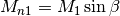
- The upstream (zone 1) Mach number
 and the flow properties
density, pressure, and temperature.
and the flow properties
density, pressure, and temperature. - The first oblique shock angle
 (between zone 1 and 2) or the
flow deflection angle
(between zone 1 and 2) or the
flow deflection angle  (across zone 1/2 and zone 2/3). Only
one of the angle is needed. The other one can be calculated from the given
one and . The calculation detail is in
(across zone 1/2 and zone 2/3). Only
one of the angle is needed. The other one can be calculated from the given
one and . The calculation detail is in
ObliqueShockRelation.calc_flow_angle()andObliqueShockRelation.calc_shock_angle().
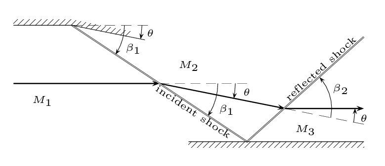
Figure 1: Oblique shock reflected from a wall
 are the Mach number in the corresponding zone 1, 2, and 3.
is the flow deflection angle.
are the Mach number in the corresponding zone 1, 2, and 3.
is the flow deflection angle.  are the
oblique shock angle behind the first and the second zone, respectively.
are the
oblique shock angle behind the first and the second zone, respectively.SOLVCON will be set up to solve this problem, and the simulated results will be compared with the analytical solution.
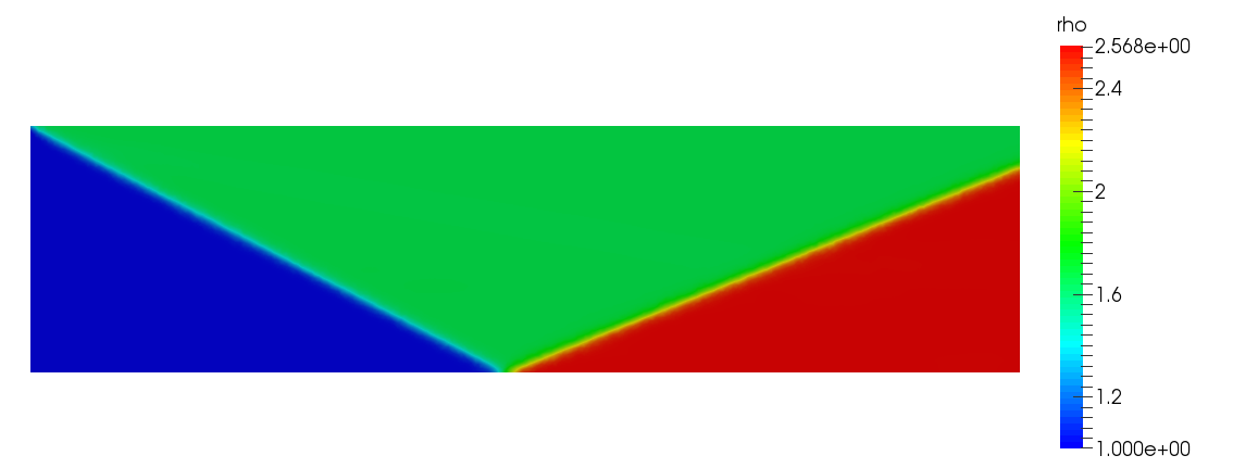
Figure 2: Simulated density (non-dimensionalized).
Driving Script
SOLVCON uses a driving script to control the numerical simulation. Its general layout is:
1 2 3 4 5 6 7 8 9 10 11 12 13 14 15 16 17 18 19 20 21 22 | #!/usr/bin/env python2.7
# The shebang above directs the operating system to look for a correct
# program to run this script.
#
# We may provide additional information here.
# Import necessary modules.
import os # Python standard library
import numpy as np # http://www.numpy.org
import solvcon as sc # SOLVCON
from solvcon.parcel import gas # A specific SOLVCON solver package we'll use
# ...
# ... other code ...
# ...
# At the end of the file.
if __name__ == '__main__':
    sc.go()
|
Every driving script has the following lines at the end of the file:
if __name__ == '__main__':
sc.go()
The if __name__ == '__main__': is a magical Python construct. It will
detect that the file is run as a script, not imported as a library (module).
Once the detection is evaluated as true, the script call a common execution
flow defined in solvcon.go(), which uses the content of the driving
script to perform the calculation.
Of course, the file has a lot of other code to set up and configure the calculation, as we’ll describe later. It’s important to note that a driving script is a valid Python program file. The Python language is good for specifying parameters the calculation needs, and as a platform to conduct useful operations much more complex than settings. Any Python module can be imported for use.
See Full Listing of the Driving Script for the driving script of this example:
$SCSRC/examples/gas/obrf/go. SOLVCON separates apart the configuration and
the execution of a simulation case. The separation is necessary for
distributed-memory parallel computing (e.g., MPI). Everything run in the
driving script is about the configuration. The execution is conducted by code
hidden from users.
To run the simulation, go to the example directory and execute the driving
script with the command run and the simulation arrangement name obrf:
$ ./go run obrf
The driving script will then run and print messages:
1 2 3 4 5 6 7 8 9 10 11 12 13 14 15 16 17 18 19 20 21 22 23 24 25 26 27 28 29 30 31 32 33 34 35 36 37 38 39 40 41 42 43 44 45 46 47 48 49 50 51 52 53 54 55 56 57 58 59 60 61 62 63 64 65 66 67 68 69 70 71 72 73 74 75 76 77 78 79 80 81 82 83 84 85 86 87 88 89 90 91 92 93 94 95 96 97 98 99 100 101 102 103 104 105 106 107 108 109 110 111 112 | ********************************************************************************
*** Start init (level 0) obrf ...
*** ****************************************************************************
*** ****************************************************************************
*** *** Start build_domain ...
*** *** ************************************************************************
*** *** mesh file: None
*** *** ************************************************************************
*** *** *** Start create_block ...
*** *** *** ********************************************************************
*** *** *** ********************************************************************
*** *** *** End create_block . Elapsed time (sec) = 0.0925829
*** *** ************************************************************************
*** *** ************************************************************************
*** *** End build_domain . Elapsed time (sec) = 0.092721
*** ****************************************************************************
*** ****************************************************************************
*** End init obrf . Elapsed time (sec) = 0.0942369
********************************************************************************
********************************************************************************
*** Start run ...
*** ****************************************************************************
*** ****************************************************************************
*** *** Start run_provide ...
*** *** ************************************************************************
*** *** ************************************************************************
*** *** End run_provide . Elapsed time (sec) = 0.000499964
*** ****************************************************************************
*** ****************************************************************************
*** *** Start run_preloop ...
*** *** ************************************************************************
*** *** Relation of reflected oblique shock:
*** *** - theta = 10.00 deg (flow angle)
*** *** - beta1 = 27.38 deg (shock angle)
*** *** - beta1 = 31.80 deg (shock angle)
*** *** - mach, rho, p, T, a (1) = 3.000 1.000 1.000 1.000 1.183
*** *** - mach, rho, p, T, a (2) = 2.505 1.655 2.054 1.242 1.318
*** *** - mach, rho, p, T, a (3) = 2.090 2.565 3.833 1.494 1.446
*** *** Steps 0/600
*** *** Block information:
*** *** [Block (2D/centroid): 565 nodes, 1592 faces (100 BC), 1028 cells]
*** *** ************************************************************************
*** *** End run_preloop . Elapsed time (sec) = 0.014756
*** ****************************************************************************
***
*** ****************************************************************************
*** *** Start run_march ...
*** *** ************************************************************************
*** *** ##################################################
*** *** Step 200/600, 0.7s elapsed, 1.4s left
*** *** CFL = 0.11/0.95 - 0.11/0.95 adjusted: 0/0/0
*** *** Performance of obrf:
*** *** 0.696783 seconds in marching solver.
*** *** 0.00348392 seconds/step.
*** *** 3.38902 microseconds/cell.
*** *** 0.29507 Mcells/seconds.
*** *** 1.18028 Mvariables/seconds.
*** *** ##################################################
*** *** Step 400/600, 1.4s elapsed, 0.7s left
*** *** CFL = 0.42/0.95 - 0.11/0.95 adjusted: 0/0/0
*** *** Performance of obrf:
*** *** 1.35721 seconds in marching solver.
*** *** 0.00339303 seconds/step.
*** *** 3.30061 microseconds/cell.
*** *** 0.302974 Mcells/seconds.
*** *** 1.2119 Mvariables/seconds.
*** *** ##################################################
*** *** Step 600/600, 2.1s elapsed, 0.0s left
*** *** CFL = 0.47/0.95 - 0.11/0.95 adjusted: 0/0/0
*** *** ************************************************************************
*** *** End run_march . Elapsed time (sec) = 2.06248
*** ****************************************************************************
***
*** ****************************************************************************
*** *** Start run_postloop ...
*** *** ************************************************************************
*** *** Probe result at Pt/poi#611(3.79306,0.358565,0)601:
*** *** - mach3 = 2.074/2.090 (error=%0.79)
*** *** - rho3 = 2.543/2.565 (error=%0.86)
*** *** - p3 = 3.824/3.833 (error=%0.23)
*** *** Performance of obrf:
*** *** 2.02795 seconds in marching solver.
*** *** 0.00337992 seconds/step.
*** *** 3.28786 microseconds/cell.
*** *** 0.30415 Mcells/seconds.
*** *** 1.2166 Mvariables/seconds.
*** *** Averaged maximum CFL = 0.945858.
*** *** Relation of reflected oblique shock:
*** *** - theta = 10.00 deg (flow angle)
*** *** - beta1 = 27.38 deg (shock angle)
*** *** - beta1 = 31.80 deg (shock angle)
*** *** - mach, rho, p, T, a (1) = 3.000 1.000 1.000 1.000 1.183
*** *** - mach, rho, p, T, a (2) = 2.505 1.655 2.054 1.242 1.318
*** *** - mach, rho, p, T, a (3) = 2.090 2.565 3.833 1.494 1.446
*** *** ************************************************************************
*** *** End run_postloop . Elapsed time (sec) = 0.00133896
*** ****************************************************************************
*** ****************************************************************************
*** *** Start run_exhaust ...
*** *** ************************************************************************
*** *** ************************************************************************
*** *** End run_exhaust . Elapsed time (sec) = 7.51019e-05
*** ****************************************************************************
*** ****************************************************************************
*** *** Start run_final ...
*** *** ************************************************************************
*** *** ************************************************************************
*** *** End run_final . Elapsed time (sec) = 9.20296e-05
*** ****************************************************************************
*** ****************************************************************************
*** End run obrf . Elapsed time (sec) = 2.07972
********************************************************************************
|
Data will be output in directory result/.
Arrangement
An arrangement sits at the center of a driving script. It’s nothing more
than a decorated Python function with a specific signature. The following
function obrf() is the main arrangement we’ll use for the shock
reflection problem:
1 2 3 4 5 6 7 8 9 | def obrf(casename, **kw):
return obrf_base(
# Required positional argument for the name of the simulation case.
casename,
# Arguments to the base configuration.
ssteps=200, psteps=4, edgelength=0.1,
gamma=1.4, density=1.0, pressure=1.0, mach=3.0, theta=10.0/180*np.pi,
# Arguments to GasCase.
time_increment=7.e-3, steps_run=600, **kw)
|
It’s typical for the arrangement function obrf() to be a thin wrapper
which calls another function (in this case, obrf_base()). It should
be noted that an arrangement function must take one and only one positional
argument: casename. All the other arguments need to be keyword.
To make the function obrf() discoverable by SOLVCON, it needs to be
registered with the decorator gas.register_arrangement
(gas was imported at the beginning of the driving
script):
@gas.register_arrangement
def obrf(casename, **kw):
# ... contents ...
The function obrf_base() does the real work of configuration:
1 2 3 4 5 6 7 8 9 10 11 12 13 14 15 16 17 18 19 20 21 22 23 24 25 26 27 28 29 30 31 32 33 34 35 36 37 38 39 40 41 42 43 44 45 46 47 48 49 50 51 52 53 54 55 56 57 58 59 60 61 62 63 64 65 66 67 68 69 | def obrf_base(
casename=None, psteps=None, ssteps=None, edgelength=None,
gamma=None, density=None, pressure=None, mach=None, theta=None, **kw):
"""
Base configuration of the simulation and return the case object.
:return: The created Case object.
:rtype: solvcon.parcel.gas.GasCase
"""
############################################################################
# Step 1: Obtain the analytical solution.
############################################################################
# Calculate the flow properties in all zones separated by the shock.
relation = ObliqueShockReflection(gamma=gamma, theta=theta, mach1=mach,
rho1=density, p1=pressure, T1=1)
############################################################################
# Step 2: Instantiate the simulation case.
############################################################################
# Create the mesh generator. Keep it for later use.
mesher = RectangleMesher(lowerleft=(0,0), upperright=(4,1),
edgelength=edgelength)
# Set up case.
cse = gas.GasCase(
# Mesh generator.
mesher=mesher,
# Mapping boundary-condition treatments.
bcmap=generate_bcmap(relation),
# Use the case name to be the basename for all generated files.
basefn=casename,
# Use `cwd`/result to store all generated files.
basedir=os.path.abspath(os.path.join(os.getcwd(), 'result')),
# Debug and capture-all.
debug=False, **kw)
############################################################################
# Step 3: Set up delayed callbacks.
############################################################################
# Field initialization and derived calculations.
cse.defer(gas.FillAnchor, mappers={'soln': gas.GasSolver.ALMOST_ZERO,
'dsoln': 0.0, 'amsca': gamma})
cse.defer(gas.DensityInitAnchor, rho=density)
cse.defer(gas.PhysicsAnchor, rsteps=ssteps)
# Report information while calculating.
cse.defer(relation.hookcls)
cse.defer(gas.ProgressHook, linewidth=ssteps/psteps, psteps=psteps)
cse.defer(gas.CflHook, fullstop=False, cflmax=10.0, psteps=ssteps)
cse.defer(gas.MeshInfoHook, psteps=ssteps)
cse.defer(ReflectionProbe, rect=mesher, relation=relation, psteps=ssteps)
# Store data.
cse.defer(gas.PMarchSave,
anames=[('soln', False, -4),
('rho', True, 0),
('p', True, 0),
('T', True, 0),
('ke', True, 0),
('M', True, 0),
('sch', True, 0),
('v', True, 0.5)],
psteps=ssteps)
############################################################################
# Final: Return the configured simulation case.
############################################################################
return cse
|
There are three steps:
- Obtain the Analytical Solution to set up all quantities for the simulation.
- Instantiate the simulation case object (of type
GasCase). TheGasCaseobject needs to know how to set up the mesh (see Mesh Generation) and the boundary-condition (BC) treatment (see BC Treatment Mapping). Section Case Instantiation will explain the details. - Configure callbacks for delayed operations by calling
defer()of the constructed simulationGasCaseobject. Section Callback Configuration will explain these callbacks.
At the end of the base function, the constructed and configured
GasCase object is returned.
Although the example has only one arrangement, it’s actually encouraged to have
multiple arrangements in a script. In this way one driving script can perform
simulations of different parameters or different kinds. Conventionally we
place the arrangement functions near the end of the driving script, and the
decorated functions (e.g., obrf()) are placed after the base (e.g.,
obrf_base()). The ordering will make the file easier to read.
Analytical Solution
To set up the numerical simulation for the shock-reflection problem, we’ll use
class ObliqueShockRelation to calculate necessary parameters by
creating a subclass of it:
1 2 3 4 5 6 7 8 9 10 11 12 13 14 15 16 17 18 19 20 21 22 23 24 25 26 27 28 29 30 31 32 33 34 35 36 37 38 39 40 41 42 43 44 45 46 47 48 49 50 | class ObliqueShockReflection(gas.ObliqueShockRelation):
def __init__(self, gamma, theta, mach1, rho1, p1, T1):
super(ObliqueShockReflection, self).__init__(gamma=gamma)
# Angles and Mach numbers.
self.theta = theta
self.mach1 = mach1
self.beta1 = beta1 = self.calc_shock_angle(mach1, theta)
self.mach2 = mach2 = self.calc_dmach(mach1, beta1)
self.beta2 = beta2 = self.calc_shock_angle(mach2, theta)
self.mach3 = mach3 = self.calc_dmach(mach2, beta2)
# Flow properties in the first zone.
self.rho1 = rho1
self.p1 = p1
self.T1 = T1
self.a1 = np.sqrt(gamma*p1/rho1)
# Flow properties in the second zone.
self.rho2 = rho2 = rho1 * self.calc_density_ratio(mach1, beta1)
self.p2 = p2 = p1 * self.calc_pressure_ratio(mach1, beta1)
self.T2 = T2 = T1 * self.calc_temperature_ratio(mach1, beta1)
self.a2 = np.sqrt(gamma*p2/rho2)
# Flow properties in the third zone.
self.rho3 = rho3 = rho2 * self.calc_density_ratio(mach2, beta2)
self.p3 = p3 = p2 * self.calc_pressure_ratio(mach2, beta2)
self.T3 = T3 = T2 * self.calc_temperature_ratio(mach2, beta2)
self.a3 = np.sqrt(gamma*p3/rho3)
def __str__(self):
msg = 'Relation of reflected oblique shock:\n'
msg += '- theta = %5.2f deg (flow angle)\n' % (self.theta/np.pi*180)
msg += '- beta1 = %5.2f deg (shock angle)\n' % (self.beta1/np.pi*180)
msg += '- beta1 = %5.2f deg (shock angle)\n' % (self.beta2/np.pi*180)
def property_string(zone):
values = [getattr(self, '%s%d' % (key, zone))
for key in 'mach', 'rho', 'p', 'T', 'a']
messages = [' %6.3f' % val for val in values]
return ''.join(messages)
msg += '- mach, rho, p, T, a (1) =' + property_string(1) + '\n'
msg += '- mach, rho, p, T, a (2) =' + property_string(2) + '\n'
msg += '- mach, rho, p, T, a (3) =' + property_string(3)
return msg
@property
def hookcls(self):
relation = self
class _ShowRelation(sc.MeshHook):
def preloop(self):
for msg in str(relation).split('\n'):
self.info(msg + '\n')
postloop = preloop
return _ShowRelation
|
For the detail of ObliqueShockRelation, see
Oblique Shock Relation.
Case Instantiation
An instance of GasCase represents a numerical
simulation using the gas module. In addition to
Mesh Generation and BC Treatment Mapping, other miscellaneous settings can
be supplied through the GasCase constructor.
Mesh Generation
An unstructured mesh is required for a SOLVCON simulation. A mesh file can be created beforehand or on-the-fly with the simulation. The example uses the latter approach. The following is an example of mesh generating function that calls Gmsh:
1 2 3 4 5 6 7 8 9 10 11 12 13 14 15 16 17 18 19 20 21 22 23 24 25 26 27 28 29 30 31 32 33 34 35 36 37 38 39 40 41 42 43 44 45 46 47 48 49 50 | class RectangleMesher(object):
"""
Representation of a rectangle and the Gmsh meshing helper.
:ivar lowerleft: (x0, y0) of the rectangle.
:type lowerleft: tuple
:ivar upperright: (x1, y1) of the rectangle.
:type upperright: tuple
:ivar edgelength: Length of each mesh cell edge.
:type edgelength: float
"""
GMSH_SCRIPT = """
// vertices.
Point(1) = {%(x1)g,%(y1)g,0,%(edgelength)g};
Point(2) = {%(x0)g,%(y1)g,0,%(edgelength)g};
Point(3) = {%(x0)g,%(y0)g,0,%(edgelength)g};
Point(4) = {%(x1)g,%(y0)g,0,%(edgelength)g};
// lines.
Line(1) = {1,2};
Line(2) = {2,3};
Line(3) = {3,4};
Line(4) = {4,1};
// surface.
Line Loop(1) = {1,2,3,4};
Plane Surface(1) = {1};
// physics.
Physical Line("upper") = {1};
Physical Line("left") = {2};
Physical Line("lower") = {3};
Physical Line("right") = {4};
Physical Surface("domain") = {1};
""".strip()
def __init__(self, lowerleft, upperright, edgelength):
assert 2 == len(lowerleft)
self.lowerleft = tuple(float(val) for val in lowerleft)
assert 2 == len(upperright)
self.upperright = tuple(float(val) for val in upperright)
self.edgelength = float(edgelength)
def __call__(self, cse):
x0, y0 = self.lowerleft
x1, y1 = self.upperright
script_arguments = dict(
edgelength=self.edgelength, x0=x0, y0=y0, x1=x1, y1=y1)
cmds = self.GMSH_SCRIPT % script_arguments
cmds = [cmd.rstrip() for cmd in cmds.strip().split('\n')]
gmh = sc.Gmsh(cmds)()
return gmh.toblock(bcname_mapper=cse.condition.bcmap)
|
BC Treatment Mapping
Boundary-condition treatments are specified by creating a dict to
map the name of the boundary to a specific BC
class.
1 2 3 4 5 6 7 8 9 10 11 12 13 14 15 16 17 18 19 20 21 22 | def generate_bcmap(relation):
# Flow properties (fp).
fpb = {
'gamma': relation.gamma, 'rho': relation.rho1,
'v2': 0.0, 'v3': 0.0, 'p': relation.p1,
}
fpb['v1'] = relation.mach1*np.sqrt(relation.gamma*fpb['p']/fpb['rho'])
fpt = fpb.copy()
fpt['rho'] = relation.rho2
fpt['p'] = relation.p2
V2 = relation.mach2 * relation.a2
fpt['v1'] = V2 * np.cos(relation.theta)
fpt['v2'] = -V2 * np.sin(relation.theta)
fpi = fpb.copy()
# BC map.
bcmap = {
'upper': (sc.bctregy.GasInlet, fpt,),
'left': (sc.bctregy.GasInlet, fpb,),
'right': (sc.bctregy.GasNonrefl, {},),
'lower': (sc.bctregy.GasWall, {},),
}
return bcmap
|
Callback Configuration
SOLVCON provides general-purpose, application-agnostic solving facilities. To describe the problem to SOLVCON, we need to provide both data (numbers) and logic (computer code) in the driving script. The supplied code will be called back at proper points while the simulation is running.
Classes MeshHook and
MeshAnchor are the fundamental constructs to make
callbacks in the sequential and parallel runtime environment, respectively.
The module gas includes useful callbacks, but we
still need to write a couple of them in the driving script.
The shock reflection problem uses three categories of callbacks.
- Initialization and calculation:
- Reporting:
ObliqueShockReflection.hookcls()ProgressHookCflHookMeshInfoHookReflectionProbe
- Output:
The order of these callbacks is important. Dependency between callbacks is allowed.
View Results
After simulation, the results are stored in directory result/ as VTK
unstructured data files that can be opened and processed by using ParaView. The result in Figure 2 was
produced in this way. Other quantities can also be visualized, e.g., the Mach
number shown in Figure 3.
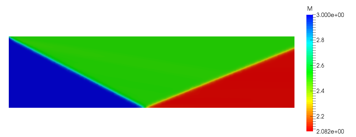
Figure 3: Mach number at the final time step of the arrangement obrf_fine.
Both of Figures 2 and 3 are
obtained with the arrangement obrf_fine.
Oblique Shock Relation
An oblique shock results from a sudden change of direction of supersonic flow.
The relations of density ( ), pressure (
 ), and temprature
(
), and temprature
( ) across the shock can be obtained analytically [Anderson03]. In
addition, two angles are defined:
) across the shock can be obtained analytically [Anderson03]. In
addition, two angles are defined:
- The angle of the oblique shock wave deflected from the upstream is
 ; the shock angle.
 - The angle of the flow behind the shock wave deflected from the upstream is
; the flow angle.
See Figure 4 for the illustration of the two angles.
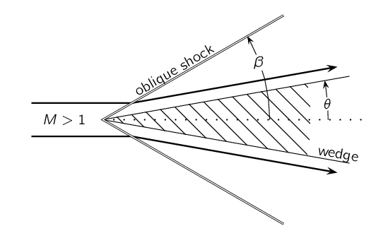
Figure 4: Oblique shock wave by a wedge
 is Mach number. is the flow deflection angle.
is the oblique shock angle.
is Mach number. is the flow deflection angle.
is the oblique shock angle.Methods of calculating the shock relations are organized in the class
ObliqueShockRelation. To obtain the relations of density
(), pressure (), and temprature (), the control
volume across the shock is emplyed, as shown in Figure
5. In the figure and in
ObliqueShockRelation, subscript 1 denotes upstream properties and
subscript 2 denotes downstream properties. Derivation of the relation uses a
rotated coordinate system  defined by the oblique shock, where
 is the unit vector normal to the shock, and
  is
the unit vector tangential to the shock. But in this document we won’t go into
the detail.
is
the unit vector tangential to the shock. But in this document we won’t go into
the detail.
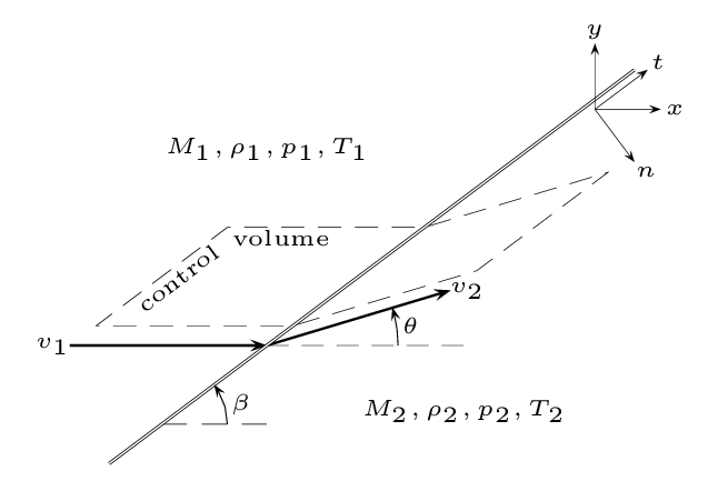
Figure 5: Properties across an oblique shock
 . Those in the downstream zone of the shock are
 .
.-
class
solvcon.parcel.gas.oblique_shock.ObliqueShockRelation(gamma)¶ Calculators of oblique shock relations.
The constructor must take the ratio of specific heat:
>>> ObliqueShockRelation() Traceback (most recent call last): ... TypeError: __init__() takes exactly 2 arguments (1 given) >>> ob = ObliqueShockRelation(gamma=1.4)
The ratio of specific heat can be accessed through the
gammaattribute:>>> ob.gamma 1.4
The object can be used to calculate shock relations. For example,
calc_density_ratio()returns the :
:>>> round(ob.calc_density_ratio(mach1=3, beta=37.8/180*np.pi), 10) 2.4204302545
The solution changes as
gammachanges:>>> ob.gamma = 1.2 >>> round(ob.calc_density_ratio(mach1=3, beta=37.8/180*np.pi), 10) 2.7793244902
-
gamma¶ Ratio of specific heat
 , dimensionless.
-
ObliqueShockRelation provides three methods to calculate the ratio
of flow properties across the shock. and are
required arguments:
With available, the shock angle can be calculated
from the flow angle , or vice versa, by using the following two
methods:
The following method calculates the downstream Mach number, with the upstream
Mach number and either of or supplied:
 :
: Listing of all methods:
calc_density_ratio()calc_pressure_ratio()calc_temperature_ratio()calc_dmach()calc_normal_dmach()calc_flow_angle()calc_flow_tangent()calc_shock_angle()calc_shock_tangent()calc_shock_tangent_aux()
-
ObliqueShockRelation.calc_density_ratio(mach1, beta)¶ Calculate the ratio of density
across an oblique shock
wave of which the angle deflected from the upstream flow is
and the upstream Mach number is :
where
 .
.This method accepts scalar:
>>> ob = ObliqueShockRelation(gamma=1.4) >>> round(ob.calc_density_ratio(mach1=3, beta=37.8/180*np.pi), 10) 2.4204302545
as well as
numpy.ndarray:>>> angle = 37.8/180*np.pi; angle = np.array([angle, angle]) >>> np.round(ob.calc_density_ratio(mach1=3, beta=angle), 10).tolist() [2.4204302545, 2.4204302545]
Parameters: - mach1 – Upstream Mach number , dimensionless.
- beta – Oblique shock angle deflected from the
upstream flow, in radian.
- mach1 – Upstream Mach number
-
ObliqueShockRelation.calc_pressure_ratio(mach1, beta)¶ Calculate the ratio of pressure
across an oblique shock wave
of which the angle deflected from the upstream flow is
and the upstream Mach number is :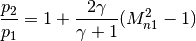
where
.This method accepts scalar:
>>> ob = ObliqueShockRelation(gamma=1.4) >>> round(ob.calc_pressure_ratio(mach1=3, beta=37.8/180*np.pi), 10) 3.7777114257
as well as
numpy.ndarray:>>> angle = 37.8/180*np.pi; angle = np.array([angle, angle]) >>> np.round(ob.calc_pressure_ratio(mach1=3, beta=angle), 10).tolist() [3.7777114257, 3.7777114257]
Parameters: - mach1 – Upstream Mach number , dimensionless.
- beta – Oblique shock angle deflected from the
upstream flow, in radian.
- mach1 – Upstream Mach number
-
ObliqueShockRelation.calc_temperature_ratio(mach1, beta)¶ Calculate the ratio of temperature
across an oblique shock wave
of which the angle deflected from the upstream flow is
and the upstream Mach number is :
where both
 and
and  are functions of
, , and . See also
are functions of
, , and . See also
calc_pressure_ratio()andcalc_density_ratio().This method accepts scalar:
>>> ob = ObliqueShockRelation(gamma=1.4) >>> round(ob.calc_temperature_ratio(mach1=3, beta=37.8/180*np.pi), 10) 1.5607602899
as well as
numpy.ndarray:>>> angle = 37.8/180*np.pi; angle = np.array([angle, angle]) >>> np.round(ob.calc_temperature_ratio(mach1=3, beta=angle), 10).tolist() [1.5607602899, 1.5607602899]
Parameters: - mach1 – Upstream Mach number , dimensionless.
- beta – Oblique shock angle deflected from the
upstream flow, in radian.
- mach1 – Upstream Mach number
-
ObliqueShockRelation.calc_dmach(mach1, beta=None, theta=None, delta=1)¶ Calculate the downstream Mach number from the upstream Mach number
and either of the shock or flow deflection angles: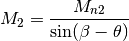
where
 is calculated from
 calc_normal_dmach()with.The method can be invoked with only either
or
:>>> ob = ObliqueShockRelation(gamma=1.4) >>> ob.calc_dmach(3, beta=0.2, theta=0.1) Traceback (most recent call last): ... ValueError: got (beta=0.2, theta=0.1), but I need to take either beta or theta >>> ob.calc_dmach(3) Traceback (most recent call last): ... ValueError: got (beta=None, theta=None), but I need to take either beta or theta
This method accepts scalar:
>>> round(ob.calc_dmach(3, beta=37.8/180*np.pi), 10) 1.9924827009 >>> round(ob.calc_dmach(3, theta=20./180*np.pi), 10) 1.9941316656
as well as
numpy.ndarray:>>> angle = 37.8/180*np.pi; angle = np.array([angle, angle]) >>> np.round(ob.calc_dmach(3, beta=angle), 10).tolist() [1.9924827009, 1.9924827009] >>> angle = 20./180*np.pi; angle = np.array([angle, angle]) >>> np.round(ob.calc_dmach(3, theta=angle), 10).tolist() [1.9941316656, 1.9941316656]
Parameters: - mach1 – Upstream Mach number , dimensionless.
- beta – Oblique shock angle deflected from the
upstream flow, in radian.
- theta – Downstream flow angle deflected from the
upstream flow, in radian.
- delta – A switching integer
 . For
. For  , the function gives the solution of strong shock,
while for
, the function gives the solution of strong shock,
while for  , it gives the solution of
weak shock. This keyword argument is only valid when
theta is given. The default value is 1.
, it gives the solution of
weak shock. This keyword argument is only valid when
theta is given. The default value is 1.
- mach1 – Upstream Mach number
-
ObliqueShockRelation.calc_normal_dmach(mach_n1)¶ Calculate the downstream Mach number from the given upstream Mach number
 , in the direction normal to the shock:
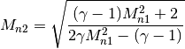
This method accepts scalar:
>>> ob = ObliqueShockRelation(gamma=1.4) >>> round(ob.calc_normal_dmach(mach_n1=3), 10) 0.4751909633
as well as
numpy.ndarray:>>> np.round(ob.calc_normal_dmach(mach_n1=np.array([3, 3])), 10).tolist() [0.4751909633, 0.4751909633]
Parameters: mach_n1 – Upstream Mach number normal to the shock
wave, dimensionless.
-
ObliqueShockRelation.calc_flow_angle(mach1, beta)¶ Calculate the downstream flow angle
deflected from the
upstream flow by using calc_flow_tangent(), in radian.This method accepts scalar:
>>> ob = ObliqueShockRelation(gamma=1.4) >>> angle = 48.25848/180*np.pi >>> round(ob.calc_flow_angle(mach1=4, beta=angle)/np.pi*180, 10) 32.0000000807
as well as
numpy.ndarray:>>> angle = 48.25848/180*np.pi; angle = np.array([angle, angle]) >>> np.round((ob.calc_flow_angle(mach1=4, beta=angle)/np.pi*180), 10).tolist() [32.0000000807, 32.0000000807]
See Example 4.6 in [Anderson03] for the forward analysis. The above is the inverse analysis.
Parameters: - mach1 – Upstream Mach number , dimensionless.
- beta – Oblique shock angle deflected from the
upstream flow, in radian.
- mach1 – Upstream Mach number
-
ObliqueShockRelation.calc_flow_tangent(mach1, beta)¶ Calculate the trigonometric tangent function
 of the
downstream flow angle deflected from the upstream flow
by using the -- relation:
of the
downstream flow angle deflected from the upstream flow
by using the -- relation: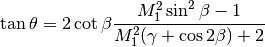
This method accepts scalar:
>>> ob = ObliqueShockRelation(gamma=1.4) >>> angle = 48.25848/180*np.pi >>> round(ob.calc_flow_tangent(mach1=4, beta=angle), 10) 0.6248693539
as well as
numpy.ndarray:>>> angle = 48.25848/180*np.pi; angle = np.array([angle, angle]) >>> np.round(ob.calc_flow_tangent(mach1=4, beta=angle), 10).tolist() [0.6248693539, 0.6248693539]
See Example 4.6 in [Anderson03] for the forward analysis. The above is the inverse analysis.
Parameters: - mach1 – Upstream Mach number , dimensionless.
- beta – Oblique shock angle deflected from the
upstream flow, in radian.
- mach1 – Upstream Mach number
-
ObliqueShockRelation.calc_shock_angle(mach1, theta, delta=1)¶ Calculate the downstream shock angle
deflected from the
upstream flow by using calc_shock_tangent(), in radian.This method accepts scalar:
>>> ob = ObliqueShockRelation(gamma=1.4) >>> angle = 32./180*np.pi >>> round(ob.calc_shock_angle(mach1=4, theta=angle, delta=1)/np.pi*180, 10) 48.2584798722
as well as
numpy.ndarray:>>> angle = np.array([angle, angle]) >>> np.round(ob.calc_shock_angle(mach1=4, theta=angle, delta=1)/np.pi*180, ... 10).tolist() [48.2584798722, 48.2584798722]
See Example 4.6 in [Anderson03] for the analysis.
Parameters: - mach1 – Upstream Mach number , dimensionless.
- theta – Downstream flow angle deflected from the
upstream flow, in radian.
- delta – A switching integer . For , the function gives the solution of strong shock,
while for , it gives the solution of
weak shock. The default value is 1.
- mach1 – Upstream Mach number
-
ObliqueShockRelation.calc_shock_tangent(mach1, theta, delta)¶ Calculate the downstream shock angle
deflected from the
upstream flow by using the alternative -- relation: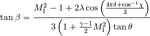
where
 and
and  are obtained internally by
calling
are obtained internally by
calling calc_shock_tangent_aux().This method accepts scalar:
>>> ob = ObliqueShockRelation(gamma=1.4) >>> angle = 32./180*np.pi >>> round(ob.calc_shock_tangent(mach1=4, theta=angle, delta=1), 10) 1.1207391858
as well as
numpy.ndarray:>>> angle = np.array([angle, angle]) >>> np.round(ob.calc_shock_tangent(mach1=4, theta=angle, delta=1), ... 10).tolist() [1.1207391858, 1.1207391858]
See Example 4.6 in [Anderson03] for the analysis.
Parameters: - mach1 – Upstream Mach number , dimensionless.
- theta – Downstream flow angle deflected from the
upstream flow, in radian.
- delta – A switching integer . For , the function gives the solution of strong shock,
while for , it gives the solution of
weak shock.
- mach1 – Upstream Mach number
-
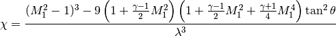
ObliqueShockRelation.calc_shock_tangent_aux(mach1, theta)¶ Calculate the
and functions used by
calc_shock_tangent():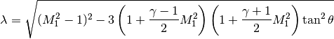
This method accepts scalar:
>>> ob = ObliqueShockRelation(gamma=1.4) >>> lmbd, chi = ob.calc_shock_tangent_aux(mach1=4, theta=32./180*np.pi) >>> round(lmbd, 10), round(chi, 10) (11.2080188412, 0.7428957121)
as well as
numpy.ndarray:>>> angle = 32./180*np.pi; angle = np.array([angle, angle]) >>> lmbd, chi = ob.calc_shock_tangent_aux(mach1=4, theta=angle) >>> np.round(lmbd, 10).tolist() [11.2080188412, 11.2080188412] >>> np.round(chi, 10).tolist() [0.7428957121, 0.7428957121]
See Example 4.6 in [Anderson03] for the analysis.
Parameters: - mach1 – Upstream Mach number , dimensionless.
- theta – Downstream flow angle deflected from the
upstream flow, in radian.
- mach1 – Upstream Mach number
Full Listing of the Driving Script
1 2 3 4 5 6 7 8 9 10 11 12 13 14 15 16 17 18 19 20 21 22 23 24 25 26 27 28 29 30 31 32 33 34 35 36 37 38 39 40 41 42 43 44 45 46 47 48 49 50 51 52 53 54 55 56 57 58 59 60 61 62 63 64 65 66 67 68 69 70 71 72 73 74 75 76 77 78 79 80 81 82 83 84 85 86 87 88 89 90 91 92 93 94 95 96 97 98 99 100 101 102 103 104 105 106 107 108 109 110 111 112 113 114 115 116 117 118 119 120 121 122 123 124 125 126 127 128 129 130 131 132 133 134 135 136 137 138 139 140 141 142 143 144 145 146 147 148 149 150 151 152 153 154 155 156 157 158 159 160 161 162 163 164 165 166 167 168 169 170 171 172 173 174 175 176 177 178 179 180 181 182 183 184 185 186 187 188 189 190 191 192 193 194 195 196 197 198 199 200 201 202 203 204 205 206 207 208 209 210 211 212 213 214 215 216 217 218 219 220 221 222 223 224 225 226 227 228 229 230 231 232 233 234 235 236 237 238 239 240 241 242 243 244 245 246 247 248 249 250 251 252 253 254 255 256 257 258 259 260 261 262 263 264 265 266 267 268 269 270 271 272 273 274 275 276 277 278 279 280 281 282 283 284 285 286 287 288 289 290 291 292 293 294 295 296 297 298 299 300 301 302 303 304 305 306 307 308 309 310 | #!/usr/bin/env python2.7
# -*- coding: UTF-8 -*-
#
# Copyright (c) 2014, Yung-Yu Chen <yyc@solvcon.net>
#
# All rights reserved.
#
# Redistribution and use in source and binary forms, with or without
# modification, are permitted provided that the following conditions are met:
#
# - Redistributions of source code must retain the above copyright notice, this
# list of conditions and the following disclaimer.
# - Redistributions in binary form must reproduce the above copyright notice,
# this list of conditions and the following disclaimer in the documentation
# and/or other materials provided with the distribution.
# - Neither the name of the SOLVCON nor the names of its contributors may be
# used to endorse or promote products derived from this software without
# specific prior written permission.
#
# THIS SOFTWARE IS PROVIDED BY THE COPYRIGHT HOLDERS AND CONTRIBUTORS "AS IS"
# AND ANY EXPRESS OR IMPLIED WARRANTIES, INCLUDING, BUT NOT LIMITED TO, THE
# IMPLIED WARRANTIES OF MERCHANTABILITY AND FITNESS FOR A PARTICULAR PURPOSE
# ARE DISCLAIMED. IN NO EVENT SHALL THE COPYRIGHT HOLDER OR CONTRIBUTORS BE
# LIABLE FOR ANY DIRECT, INDIRECT, INCIDENTAL, SPECIAL, EXEMPLARY, OR
# CONSEQUENTIAL DAMAGES (INCLUDING, BUT NOT LIMITED TO, PROCUREMENT OF
# SUBSTITUTE GOODS OR SERVICES; LOSS OF USE, DATA, OR PROFITS; OR BUSINESS
# INTERRUPTION) HOWEVER CAUSED AND ON ANY THEORY OF LIABILITY, WHETHER IN
# CONTRACT, STRICT LIABILITY, OR TORT (INCLUDING NEGLIGENCE OR OTHERWISE)
# ARISING IN ANY WAY OUT OF THE USE OF THIS SOFTWARE, EVEN IF ADVISED OF THE
# POSSIBILITY OF SUCH DAMAGE.
"""
This is an example for solving the problem of oblique shock reflection.
"""
import os # Python standard library
import numpy as np # http://www.numpy.org
import solvcon as sc # SOLVCON
from solvcon.parcel import gas # A specific SOLVCON solver package we'll use
class ObliqueShockReflection(gas.ObliqueShockRelation):
def __init__(self, gamma, theta, mach1, rho1, p1, T1):
super(ObliqueShockReflection, self).__init__(gamma=gamma)
# Angles and Mach numbers.
self.theta = theta
self.mach1 = mach1
self.beta1 = beta1 = self.calc_shock_angle(mach1, theta)
self.mach2 = mach2 = self.calc_dmach(mach1, beta1)
self.beta2 = beta2 = self.calc_shock_angle(mach2, theta)
self.mach3 = mach3 = self.calc_dmach(mach2, beta2)
# Flow properties in the first zone.
self.rho1 = rho1
self.p1 = p1
self.T1 = T1
self.a1 = np.sqrt(gamma*p1/rho1)
# Flow properties in the second zone.
self.rho2 = rho2 = rho1 * self.calc_density_ratio(mach1, beta1)
self.p2 = p2 = p1 * self.calc_pressure_ratio(mach1, beta1)
self.T2 = T2 = T1 * self.calc_temperature_ratio(mach1, beta1)
self.a2 = np.sqrt(gamma*p2/rho2)
# Flow properties in the third zone.
self.rho3 = rho3 = rho2 * self.calc_density_ratio(mach2, beta2)
self.p3 = p3 = p2 * self.calc_pressure_ratio(mach2, beta2)
self.T3 = T3 = T2 * self.calc_temperature_ratio(mach2, beta2)
self.a3 = np.sqrt(gamma*p3/rho3)
def __str__(self):
msg = 'Relation of reflected oblique shock:\n'
msg += '- theta = %5.2f deg (flow angle)\n' % (self.theta/np.pi*180)
msg += '- beta1 = %5.2f deg (shock angle)\n' % (self.beta1/np.pi*180)
msg += '- beta1 = %5.2f deg (shock angle)\n' % (self.beta2/np.pi*180)
def property_string(zone):
values = [getattr(self, '%s%d' % (key, zone))
for key in 'mach', 'rho', 'p', 'T', 'a']
messages = [' %6.3f' % val for val in values]
return ''.join(messages)
msg += '- mach, rho, p, T, a (1) =' + property_string(1) + '\n'
msg += '- mach, rho, p, T, a (2) =' + property_string(2) + '\n'
msg += '- mach, rho, p, T, a (3) =' + property_string(3)
return msg
@property
def hookcls(self):
relation = self
class _ShowRelation(sc.MeshHook):
def preloop(self):
for msg in str(relation).split('\n'):
self.info(msg + '\n')
postloop = preloop
return _ShowRelation
class RectangleMesher(object):
"""
Representation of a rectangle and the Gmsh meshing helper.
:ivar lowerleft: (x0, y0) of the rectangle.
:type lowerleft: tuple
:ivar upperright: (x1, y1) of the rectangle.
:type upperright: tuple
:ivar edgelength: Length of each mesh cell edge.
:type edgelength: float
"""
GMSH_SCRIPT = """
// vertices.
Point(1) = {%(x1)g,%(y1)g,0,%(edgelength)g};
Point(2) = {%(x0)g,%(y1)g,0,%(edgelength)g};
Point(3) = {%(x0)g,%(y0)g,0,%(edgelength)g};
Point(4) = {%(x1)g,%(y0)g,0,%(edgelength)g};
// lines.
Line(1) = {1,2};
Line(2) = {2,3};
Line(3) = {3,4};
Line(4) = {4,1};
// surface.
Line Loop(1) = {1,2,3,4};
Plane Surface(1) = {1};
// physics.
Physical Line("upper") = {1};
Physical Line("left") = {2};
Physical Line("lower") = {3};
Physical Line("right") = {4};
Physical Surface("domain") = {1};
""".strip()
def __init__(self, lowerleft, upperright, edgelength):
assert 2 == len(lowerleft)
self.lowerleft = tuple(float(val) for val in lowerleft)
assert 2 == len(upperright)
self.upperright = tuple(float(val) for val in upperright)
self.edgelength = float(edgelength)
def __call__(self, cse):
x0, y0 = self.lowerleft
x1, y1 = self.upperright
script_arguments = dict(
edgelength=self.edgelength, x0=x0, y0=y0, x1=x1, y1=y1)
cmds = self.GMSH_SCRIPT % script_arguments
cmds = [cmd.rstrip() for cmd in cmds.strip().split('\n')]
gmh = sc.Gmsh(cmds)()
return gmh.toblock(bcname_mapper=cse.condition.bcmap)
def generate_bcmap(relation):
# Flow properties (fp).
fpb = {
'gamma': relation.gamma, 'rho': relation.rho1,
'v2': 0.0, 'v3': 0.0, 'p': relation.p1,
}
fpb['v1'] = relation.mach1*np.sqrt(relation.gamma*fpb['p']/fpb['rho'])
fpt = fpb.copy()
fpt['rho'] = relation.rho2
fpt['p'] = relation.p2
V2 = relation.mach2 * relation.a2
fpt['v1'] = V2 * np.cos(relation.theta)
fpt['v2'] = -V2 * np.sin(relation.theta)
fpi = fpb.copy()
# BC map.
bcmap = {
'upper': (sc.bctregy.GasInlet, fpt,),
'left': (sc.bctregy.GasInlet, fpb,),
'right': (sc.bctregy.GasNonrefl, {},),
'lower': (sc.bctregy.GasWall, {},),
}
return bcmap
class ReflectionProbe(gas.ProbeHook):
"""
Place a probe for the flow properties in the reflected region.
"""
def __init__(self, cse, **kw):
"""
:param relation: Instruct shock relations.
:type relation: ObliqueShockReflection
:param rect: Instruct the mesh rectangle.
:type rect: RectangleMesher
"""
rect = kw.pop('rect')
self.relation = relation = kw.pop('relation')
factor = kw.pop('factor', 0.9)
# Detemine location.
theta = relation.theta
beta1 = relation.beta1
beta2 = relation.beta2
x0, y0 = rect.lowerleft
x1, y1 = rect.upperright
lgh = (y1-y0) / np.tan(beta1)
hgt = factor * (x1-x0-lgh) * np.tan((beta2-theta)/2)
lgh = factor * (x1-x0-lgh) + lgh
poi = ('poi', x0+lgh, y0+hgt, 0.0)
# Call super.
kw['coords'] = (poi,)
kw['speclst'] = ['M', 'rho', 'p']
super(ReflectionProbe, self).__init__(cse, **kw)
def postloop(self):
super(ReflectionProbe, self).postloop()
rel = self.relation
self.info('Probe result at %s:\n' % self.points[0])
M, rho, p = self.points[0].vals[-1][1:]
self.info('- mach3 = %.3f/%.3f (error=%%%.2f)\n' % (
M, rel.mach3, abs((M-rel.mach3)/rel.mach3)*100))
self.info('- rho3 = %.3f/%.3f (error=%%%.2f)\n' % (
rho, rel.rho3, abs((rho-rel.rho3)/rel.rho3)*100))
self.info('- p3 = %.3f/%.3f (error=%%%.2f)\n' % (
p, rel.p3, abs((p-rel.p3)/rel.p3)*100))
def obrf_base(
casename=None, psteps=None, ssteps=None, edgelength=None,
gamma=None, density=None, pressure=None, mach=None, theta=None, **kw):
"""
Base configuration of the simulation and return the case object.
:return: The created Case object.
:rtype: solvcon.parcel.gas.GasCase
"""
############################################################################
# Step 1: Obtain the analytical solution.
############################################################################
# Calculate the flow properties in all zones separated by the shock.
relation = ObliqueShockReflection(gamma=gamma, theta=theta, mach1=mach,
rho1=density, p1=pressure, T1=1)
############################################################################
# Step 2: Instantiate the simulation case.
############################################################################
# Create the mesh generator. Keep it for later use.
mesher = RectangleMesher(lowerleft=(0,0), upperright=(4,1),
edgelength=edgelength)
# Set up case.
cse = gas.GasCase(
# Mesh generator.
mesher=mesher,
# Mapping boundary-condition treatments.
bcmap=generate_bcmap(relation),
# Use the case name to be the basename for all generated files.
basefn=casename,
# Use `cwd`/result to store all generated files.
basedir=os.path.abspath(os.path.join(os.getcwd(), 'result')),
# Debug and capture-all.
debug=False, **kw)
############################################################################
# Step 3: Set up delayed callbacks.
############################################################################
# Field initialization and derived calculations.
cse.defer(gas.FillAnchor, mappers={'soln': gas.GasSolver.ALMOST_ZERO,
'dsoln': 0.0, 'amsca': gamma})
cse.defer(gas.DensityInitAnchor, rho=density)
cse.defer(gas.PhysicsAnchor, rsteps=ssteps)
# Report information while calculating.
cse.defer(relation.hookcls)
cse.defer(gas.ProgressHook, linewidth=ssteps/psteps, psteps=psteps)
cse.defer(gas.CflHook, fullstop=False, cflmax=10.0, psteps=ssteps)
cse.defer(gas.MeshInfoHook, psteps=ssteps)
cse.defer(ReflectionProbe, rect=mesher, relation=relation, psteps=ssteps)
# Store data.
cse.defer(gas.PMarchSave,
anames=[('soln', False, -4),
('rho', True, 0),
('p', True, 0),
('T', True, 0),
('ke', True, 0),
('M', True, 0),
('sch', True, 0),
('v', True, 0.5)],
psteps=ssteps)
############################################################################
# Final: Return the configured simulation case.
############################################################################
return cse
@gas.register_arrangement
def obrf(casename, **kw):
    return obrf_base(
        # Required positional argument for the name of the simulation case.
        casename,
        # Arguments to the base configuration.
        ssteps=200, psteps=4, edgelength=0.1,
        gamma=1.4, density=1.0, pressure=1.0, mach=3.0, theta=10.0/180*np.pi,
        # Arguments to GasCase.
        time_increment=7.e-3, steps_run=600, **kw)
@gas.register_arrangement
def obrf_fine(casename, **kw):
return obrf_base(
casename,
ssteps=200, psteps=4, edgelength=0.02,
gamma=1.4, density=1.0, pressure=1.0, mach=3.0, theta=10.0/180*np.pi,
time_increment=1.e-3, steps_run=4000, **kw)
if __name__ == '__main__':
sc.go()
# vim: set ff=unix fenc=utf8 ft=python ai et sw=4 ts=4 tw=79:
|