Solver Architecture
SOLVCON is built upon two keystones: (i) unstructured meshes for spatial discretization and (ii) two-level loop structure of partial differential equation (PDE) solvers.
Unstructured Meshes
We usually discretize the spatial domain of interest before solving PDEs with digital computers. The discretized space is called a mesh [Mavriplis97]. When discretization is done by exploiting regularity in space, like cutting along each of the Cartesian coordinate axes, the discretized space is called a structured mesh. If the discretization does not follow any spatial order, we call the spatial domain an unstructured mesh. Both meshing strategies have their strength and weakness. Sometimes a structured mesh is also call a grid. Numerical methods that rely on spatial discretization are called mesh-based or grid-based. Most PDE-solving methods in production uses are mesh-based, but meshless methods have their advantages.
To accommodate complex geometry, SOLVCON chose to use unstructured meshes of mixed elements. Because no structure is assumed for the geometry to be modeled, the mesh can be automatically generated by using computer programs. For example, the following image shows a triangular mesh of a two-dimensional irregular domain:
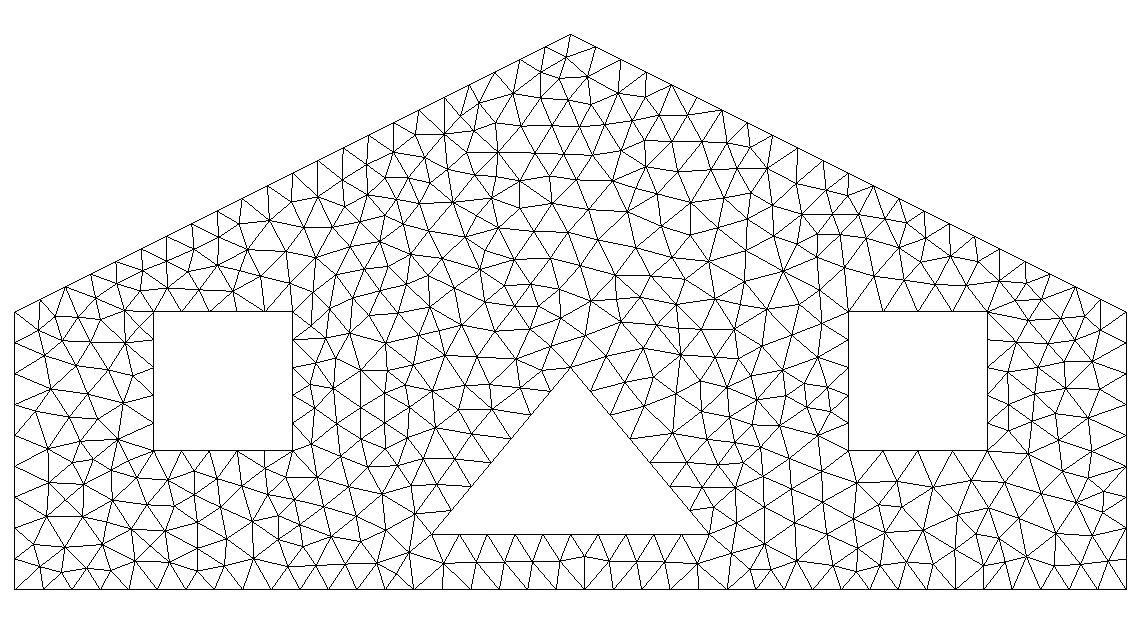
Figure 1: Two-dimensional sample mesh
which is generated by using the Gmsh commands listed in ustmesh_2d_sample.geo. On the other hand, creation of structured meshes often needs a large amount of manual operations and will not be discussed in this document.
In SOLVCON, we assume a mesh is fully covered by a finite number of non-overlapping sub-regions, and only composed by these sub-regions. The sub-regions are called mesh elements. In one-dimensional space, SOLVCON also defines one type of mesh elements, line, as shown in Figure One-dimensional mesh element.
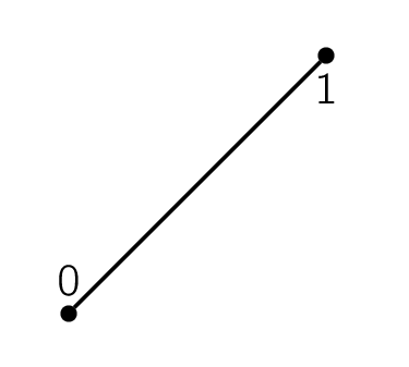
Figure 2: One-dimensional mesh element
SOLVCON allows two types of two-dimensional mesh elements, quadrilaterals and triangles, as shown in Figure Two-dimensional mesh elements, and four types of three-dimensional mesh elements, hexahedra, tetrahedra, prisms, and pyramids, as shown in Figure Three-dimensional mesh elements.

Figure 3: Two-dimensional mesh elements

Figure 4: Three-dimensional mesh elements
The numbers annotated in the figures are the order of the vertices of the
elements. A SOLVCON mesh can be a mixture of elements of the same dimension,
although it is often composed of one type of element. Two modules provide the
support of the meshes: (i) solvcon.block defines and manages
various look-up tables that form the data structure of the mesh in Python, and
(ii) solvcon.mesh serves as the interface of the mesh data in C.
Entities
Before explaining the data structure of the meshes, we need to introduce some basic terminologies and definitions. In SOLVCON, a cell means a mesh element. The dimensionality of a cell equals to that of the mesh it belongs to, e.g., a two-dimensional mesh is composed by two-dimensional cells. A cell is assumed to be concave, and enclosed by a set of faces. The dimensionality of a face is one less than that of a cell. A face is also assumed to be concave, and formed by connecting a sequence of nodes. The dimensionality of a node is at least one less than that of a face. Cells, faces, and nodes are the basic constructs, which we call entities, of a SOLVCON mesh.
Defining the term “entity” for SOLVCON facilitates a unified treatment of two- and three-dimensional meshes and the corresponding solvers [1]. A cell can be either two- or three-dimensional, and the associated faces become one- or two-dimensional, respectively. Because a face is either one- or two-dimensional, it can always be formed by a sequence of points, which is zero-dimensional. In this treatment, a point is equivalent to a node defined in the previous passage.
Take the two-dimensional mesh shown above as an example, triangular elements are used as the cells. The triangles are formed by three lines (one-dimensional shapes), which are the faces. Each line has two points (zero-dimensional). If we have a three-dimensional mesh composed by hexahedral cells, then the faces should be quadrilaterals (two-dimensional shapes).
All the mesh elements supported by SOLVCON are listed in the following table. The first column is the name of the element, and the second column is the type ID used in SOLVCON. The third column lists the dimensionality. The fourth, fifth, and sixth columns show the number of zero-, one-, and two-dimensional sub-entities belong to the element type, respectively. Note that the terms “point” and “line” appear in both the first row and first column, for they are the only element type in the space of the corresponding dimensionality.
| Name | Type | Dim | Point# | Line# | Surface# |
|---|---|---|---|---|---|
| Point | 0 | 0 | 0 | 0 | 0 |
| Line | 1 | 1 | 2 | 0 | 0 |
| Quadrilateral | 2 | 2 | 4 | 4 | 0 |
| Triangle | 3 | 2 | 3 | 3 | 0 |
| Hexahedron | 4 | 3 | 8 | 12 | 6 |
| Tetrahedron | 5 | 3 | 4 | 4 | 4 |
| Prism | 6 | 3 | 6 | 9 | 5 |
| Pyramid | 7 | 3 | 5 | 8 | 5 |
Although SOLVCON doesn’t support one-dimensional solvers, for completeness, we define the relation between one-dimensional cells (lines) and their sub-entities as:
| Shape (type) | Face | = Point |
|---|---|---|
| Line (0) | 0 |  0 0 |
| 1 | 1 |
That is, as shown in Figure One-dimensional mesh element, a one-dimensional “cell” (line)
has two “faces”, which are essentially point 0 and point 1. Symbol
indicates a point.
It will be more practical to illustrate the relation between two-dimensional cells and their sub-entities in a table (see Figure Two-dimensional mesh elements for point locations):
| Shape (type) | Face | = Line formed by points |
|---|---|---|
| Quadrilateral (2) | 0 |  0 1 0 1 |
| 1 | 1 2 |
|
| 2 | 2 3 |
|
| 3 | 3 0 |
|
| Triangle (3) | 0 | 0 1 |
| 1 | 1 2 |
|
| 2 | 2 0 |
Symbol indicates a line. The orientation of lines of each
two-dimensional shape is defined to follow the right-hand rule. The shape
enclosed by the lines has an area normal vector points to the direction of
 (outward paper/screen).
The relation between three-dimensional cells and their sub-entities is defined in the table (see Figure Three-dimensional mesh elements for point locations):
| Shape (type) | Face | = Surface formed by points |
|---|---|---|
| Hexahedron (4) | 0 |  0 3 2 1 0 3 2 1 |
| 1 | 1 2 6 5 |
|
| 2 | 4 5 6 7 |
|
| 3 | 0 4 7 3 |
|
| 4 | 0 1 5 4 |
|
| 5 | 2 3 7 6 |
|
| Tetrahedron (5) | 0 |  0 2 1 0 2 1 |
| 1 | 0 1 3 |
|
| 2 | 0 3 2 |
|
| 3 | 1 2 3 |
|
| Prism (6) | 0 | 0 1 2 |
| 1 | 3 5 4 |
|
| 2 | 0 3 4 1 |
|
| 3 | 0 2 5 3 |
|
| 4 | 1 4 5 2 |
|
| Pyramid (7) | 0 | 0 4 3 |
| 1 | 1 4 0 |
|
| 2 | 2 4 1 |
|
| 3 | 3 4 2 |
|
| 4 | 0 3 2 1 |
Symbol indicates a quadrilateral, while symbol
indicates a triangle.
Because a face is associated to two adjacent cells unless it’s a boundary face, it needs to identify to which cell it belongs, and to which cell it is neighbor. The area normal vector of a face is always point from the belonging cell to neighboring cell. The same rule applies to faces of two-dimensional meshes (lines) too.
Data Structure Defined in solvcon.block
Real data of unstructured meshes are stored in module
solvcon.block. A simple table for all element types is defined as
elemtype:
-
solvcon.block.elemtype¶ A
numpy.ndarrayobject of shape (8, 5) and typeint32. This array is a reference table for element types in SOLVCON. The content is shown in the first table in Section Entities. Each row represents an element type. The first column is the index of the element type, the second the dimensionality, the third column the number of points, the fourth the number lines, and the fifth the number of surfaces.
Class Block contains descriptive information, look-up tables, and
other miscellaneous information for a SOLVCON mesh. There are three steps
required to fully construct a Block object: (i) instantiation, (ii)
definition, and (iii) build-up. In the first step, when instantiating an
object, shape information must be provided to the constructor to allocate
arrays for look-up tables:
from solvcon.block import Block
blk = Block(ndim=2, nnode=4, ncell=3)
Second, we fill the definition of the look-up tables into the object. We at least need to provide the node coordinates and the node lists of cells:
blk.ndcrd[:,:] = (0,0), (-1,-1), (1,-1), (0,1)
blk.cltpn[:] = 3
blk.clnds[:,:4] = (3, 0,1,2), (3, 0,2,3), (3, 0,3,1)
Third and finally, we build up the rest of the object by calling:
blk.build_interior()
blk.build_boundary()
blk.build_ghost()
By running the additional code, the block can be saved as a VTK file for viewing:
from solvcon.io.vtkxml import VtkXmlUstGridWriter
iodev = VtkXmlUstGridWriter(blk)
iodev.write('block_2d_sample.vtu')
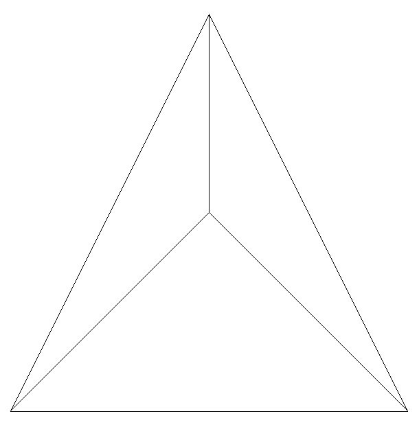
Figure 5: A simple Block object
-
class
solvcon.block.Block(ndim=0, nnode=0, nface=0, ncell=0, nbound=0, use_incenter=False)¶ This class represents the unstructured meshes used in SOLVCON. As such, in SOLVCON, an unstructured mesh is also called a block. The following six attributes can be passed into the constructor.
ndim,nnode, andncellneed to be non-zero to instantiate a valid block.nfaceandnboundmight be different to the given value after building up the object.use_incenteris an optional flag.-
nbound¶ Type: intTotal number of boundary faces or ghost cells of this mesh. Read only after instantiation.
-
use_incenter¶ Type: boolIndicates calculating incenters instead of centroids for cells. Default is
False(using centroids of cells).
To construct a block object, SOLVCON needs to know the dimensionalities (
ndim), the number of nodes (nnode), faces (nface), and cells (ncell), and the number of boundary faces (nbound) of the mesh. These keyword parameters are taken to initialize the following properties:The meshes are mainly defined by three sets of look-up tables (arrays). The first set is the geometry arrays, which store the coordinate values of mesh elements:
-
ndcrd¶ Coordinates of nodes. It’s a two-dimensional
numpy.ndarrayarray of shape (nnode,ndim) of typefloat64.
-
fccnd¶ Centroids of faces. It’s a two-dimension
numpy.ndarrayof shape (nface,ndim) of typefloat64.
-
fcnml¶ Unit normal vectors of faces. It’s a two-dimension
numpy.ndarrayof shape (nface,ndim) of typefloat64.
-
fcara¶ Areas of faces. The value should always be non-negative. It’s a one-dimension
numpy.ndarrayof shape (nface,) of typefloat64.
-
clcnd¶ Centroids of cells. It’s a two-dimension
numpy.ndarrayof shape (ncell,ndim) of typefloat64.
The second set is the meta-data or type data arrays:
-
clgrp¶ Group ID of cells. It’s a one-dimensional
numpy.ndarrayof shape (ncell,) of typeint32. For a newBlockobject, it should be initialized with-1.
The third and last set is the connectivity arrays:
-
fcnds¶ Lists of the nodes of each face. It’s a two-dimensional
numpy.ndarrayof shape (nface,FCMND+1) and typeint32.
-
fccls¶ Lists of the cells connected by each face. It’s a two-dimensional
numpy.ndarrayof shape (nface, 4) and typeint32.
-
clnds¶ Lists of the nodes of each cell. It’s a two-dimensional
numpy.ndarrayof shape (ncell,CLMND+1) and typeint32.
-
clfcs¶ Lists of the faces of each cell. It’s a two-dimensional
numpy.ndarrayof shape (ncell,CLMFC+1) and typeint32.
Every look-up array has two associated arrays distinguished by different prefixes: (i)
gst(denoting for “ghost”) and (ii)sh(denoting for “shared”). SOLVCON uses the technique of ghost cells to treat boundary conditions [Mavriplis97], and thegstarrays store the information for ghost cells. However, to facilitate efficient indexing in solvers, each of the ghost arrays should be put in a continuous block of memory adjacent to its interior counterpart. In SOLVCON, thesharrays are the continuous memory blocks for both ghost and interior look-up tables, and a pair ofgstand normal arrays is simply the views of two consecutive, non-overlapping sub-regions of a memory block. More details of the technique of ghost cells will be given in modulesolvcon.mesh.There are some attributes associated with ghost cells:
-
ngstnode¶ Type: intNumber of nodes only associated with ghost cells. Only valid after build-up. Read only.
-
ngstface¶ Type: intNumber of faces only associated with ghost cells. Only valid after build-up. Read only.
Three arrays need to be defined before we can build up a
Blockobject: (i)ndcrd, (ii)cltpn, and (iii)clnds. With these information,build_interior()builds up the interior arrays for aBlockobject.build_boundary()then organizes the information for boundary conditions. Finally,build_ghost()builds up the shared and ghost arrays for theBlockobject. Only after the build-up process, theBlockobject can be used by solvers.-
build_interior()¶ Returns: Nothing. Building up a
Blockobject includes two steps. First, the method extracts arraysclfcs,fctpn,fcnds, andfcclsfrom the defined arrayscltpnandclnds. If the number of extracted faces is not the same as that passed into the constructor, arrays related to faces are recreated.Second, the method calculates the geometry information and fills the corresponding arrays.
-
build_boundary(unspec_type=None, unspec_name='unspecified')¶ Parameters: Returns: Nothing.
This method iterates over each of the
solvcon.boundcond.BCobjects listed inbclistto collect boundary-condition information and build boundary faces. If a face belongs to only one cell (i.e., has no neighboring cell), it is regarded as a boundary face.Unspecified boundary faces will be collected to form an additional
solvcon.boundcond.BCobject. It setsbndfcsfor later use bybuild_ghost().
-
build_ghost()¶ Returns: Nothing. This method creates the shared arrays, calculates the information for ghost cells, and reassigns interior arrays as the right portions of the shared arrays.
A
Blockobject also contains three instance variables for boundary-condition treatments:-
bclist¶ Type: listThe list of associated
solvcon.boundcond.BCobjects.
-
bndfcs¶ Type: numpy.ndarrayThe array is of shape (
nbound, 2) and typeint32. Each row contains the data for a boundary face. The first column is the 0-based index of the face, while the second column is the serial number of the associatedsolvcon.boundcond.BCobject.
-
create_msh()¶ Returns: An object contains the sc_mesh_tvariable for C code to use data in theBlockobject.Return type: solvcon.mesh.MeshThe following code shows how and when to use this method:
>>> blk = Block(ndim=2, nnode=4, nface=6, ncell=3, nbound=3)
>>> blk.ndcrd[:,:] = (0,0), (-1,-1), (1,-1), (0,1)
>>> blk.cltpn[:] = 3
>>> blk.clnds[:,:4] = (3, 0,1,2), (3, 0,2,3), (3, 0,3,1)
>>> blk.build_interior()
>>> # it's OK to get a msh when its content is still invalid.
>>> msh = blk.create_msh()
>>> blk.build_boundary()
>>> blk.build_ghost()
>>> # now the msh is valid for the blk is fully built-up.
>>> msh = blk.create_msh()
-
In class Block there are also useful constants defined:
Low-Level Interface to C Defined in solvcon.mesh
Although it is convenient to have data structure defined in the Python module
solvcon.block, kernel of numerical methods are usually implemented in
C. To bridge Python and C, we use Cython to write an
interfacing module solvcon.mesh. This module enables C code to use
the mesh data held by a solvcon.block.Block object, and allows Python
to use those C functions.
A header file mesh.h contains the essential declarations to use the mesh
data:
-
sc_mesh_t¶ This
structis the counterpart of the Python classsolvcon.block.Blockin C. It contains four sections of fields in order.The first field section is for shape. These fields correspond to the instance properties (attributes) in
solvcon.block.Blockof the same names:-
int
ndim
-
int
nnode
-
int
nface
-
int
ncell
-
int
nbound
-
int
ngstnode
-
int
ngstface
-
int
ngstcell
The second field section is for geometry arrays. These fields correspond to the instance variables (attributes) in
solvcon.block.Blockof the same names:Note
All arrays in
sc_mesh_tare shared arrays but the pointers point to the start of their interior portion. In this way, access to ghost information can be efficiently done by using negative indices of nodes, faces, and cells in the first dimension of these arrays. But negative indices in higher dimensions of the arrays is meaningless.-
double*
ndcrd
-
double*
fccnd
-
double*
fcnml
-
double*
fcara
-
double*
clcnd
-
double*
clvol
The third field section is for type/meta arrays. These fields correspond to the instance variables (attributes) in
solvcon.block.Blockof the same names:-
int*
fctpn
-
int*
cltpn
-
int*
clgrp
The fourth and final field section is for connectivity arrays. These fields correspond to the instance variables (attributes) in
solvcon.block.Blockof the same names:-
int*
fcnds
-
int*
fccls
-
int*
clnds
-
int*
clfcs
-
int
The SOLVCON C library (libsolvcon.a) contains five mesh-related functions
that are used internally in Mesh. These functions are not meant to
be part of the interface, but can be a reference about the usage of
sc_mesh_t:
-
int
sc_mesh_extract_faces_from_cells(sc_mesh_t *msd, int mface, int *pnface, int *clfcs, int *fctpn, int *fcnds, int *fccls)¶ This function extracts interior faces from the node lists of the cells given in the first argument
msd. The second argumentmfaceis also an input, which sets the maximum value of possible number of faces to be extracted.The rest of the arguments is outputs. The arrays pointed by the last four arguments need to be pre-allocated with appropriate size or the memory will be corrupted.
-
int
sc_mesh_calc_metric(sc_mesh_t *msd, int use_incenter)¶ This function calculates the geometry information and stores the calculated values into the arrays specified in
msd. The second argumentuse_incenteris a flag. When it is set to1, the function calculates and stores the incenter of the cells. Otherwise, the function calculates and stores the centroids of the cells.
-
void
sc_mesh_build_ghost(sc_mesh_t *msd, int *bndfcs)¶ Build all information for ghost cells by mirroring information from interior cells. The arrays in the first argument
msdwill be altered, but data in the second argumentbndfcswill remain intact. The action includes:- Define indices and build connectivities for ghost nodes, faces, and cells. In the same loop, mirror the coordinates of interior nodes to ghost nodes.
- Compute center coordinates for faces for ghost cells.
- Compute normal vectors and areas for faces for ghost cells.
- Compute center coordinates for ghost cells.
- Compute volume for ghost cells.
It should be noted that all the geometry, type/meta and connectivity data used in this function are SHARED arrays rather than interior arrays. The indices for ghost information should be carefully treated. All the ghost indices are negative in shared arrays.
-
int
sc_mesh_build_rcells(sc_mesh_t *msd, int *rcells, int *rcellno)¶ This is a utility function used by
Mesh.create_csr(). The first argumentmsdis input and will not be changed, and the output will be write to the second and third arguments,rcellsandrcellno. Sufficient memory must be pre-allocated for the output arrays before calling or memory can be corrupted.
-
int
sc_mesh_build_csr(sc_mesh_t *msd, int *rcells, int *adjncy)¶ This is a utility function used by
Mesh.create_csr(). The first argumentmsdand the second argumentrcellsare input and will not be changed, while the third argumentadjncyis output. Sufficient memory must be pre-allocated for the output array before calling or memory can be corrupted.
A Python class Mesh is written by using Cython to convert a
Python-space solvcon.block.Block object into a sc_mesh_t
struct variable for use in C. This class is meant to be subclassed to
implement the core number-crunching algorithm of a numerical method. In
addition, this class also provides functionalities that need the C utility
functions listed above.
-
class
solvcon.mesh.Mesh¶ This class associates the C functions for mesh operations to the mesh data and exposes the functions to Python.
-
setup_mesh(blk)¶ Parameters: blk ( solvcon.block.Block) – The block object that supplies the information.
-
extract_faces_from_cells(max_nfc)¶ Parameters: max_nfc (C int) – Maximum value of possible number of faces to be extracted.Returns: Four interior numpy.ndarrayforsolvcon.block.Block.clfcs,solvcon.block.Block.fctpn,solvcon.block.Block.fcnds, andsolvcon.block.Block.fccls.Internally calls
sc_mesh_extract_face_from_cells().
-
calc_metric()¶ Returns: Nothing. Calculates geometry information including normal vector and area of faces, and centroid/incenter coordinates and volume of cells. Internally calls
sc_mesh_calc_metric().
-
build_ghost()¶ Returns: Nothing. Builds data for ghost cells. Internally calls
sc_mesh_build_ghost().
-
create_csr()¶ Returns: xadj, adjncy Return type: tuple of numpy.ndarrayBuilds the connectivity graph in the CSR (compressed storage format) used by SCOTCH/METIS. Internally calls
sc_mesh_build_rcells()andsc_mesh_build_csr().
-
partition(npart, vwgtarr=None)¶ Parameters: - npart (C
int) – Number of parts to be partitioned to. - vwgtarr (
numpy.ndarray) – vwgt weighting settings. Default isNone.
Returns: A 2-tuple of (i) number of cut edges for the partitioning and (ii) a
numpy.ndarrayof shape (solvcon.block.Block.ncell,) and typeint32that indicates the partition number of each cell in the mesh.Return type: int,numpy.ndarrayInternally calls
METIS_PartGraphKway()of the SCOTCH library for mesh partitioning.- npart (C
-
Numerical Code
The numerical calculations in SOLVCON rely on exploiting a two-level loop
structure, i.e., the temporal loop and the spatial loops. For time-accurate
solvers, there is always an outer loop that coordinates the time-marching. The
outer loop is called the temporal loop, and it should be implemented in
subclasses of MeshCase. Inside the
temporal loop, there can be one or many inner loops that calculate the new
values of the fields. The inner loops are called the spatial loops, and they
should be implemented in subclasses of MeshSolver.
The outer temporal loop is more responsible for coordinating, while the inner
spatial loops is closer to numerical algorithms. These two levels allow us to
segregate code. An object of MeshCase can
be seen as the realization of a simulation case in SOLVCON (as a convention the
object’s name should contain or just be cse). Code in MeshCase is mainly about obtaining settings, input and output,
and provision of the execution environment. On the other hand, we implement
the numerical algorithm in MeshSolver
to manipulate the field data (as a convention the object’s name should contain
or just be svr). Its code shouldn’t involve input nor output (excepting
that for debugging) but needs to take parallelism into account.
Code for data processing should go to MeshHook (as a convention the objects should be named with
hok), which is the companion of MeshCase. Code that processes data close to numerical methods
should go to MeshAnchor (as a
convention the objects should be named with ank), which is the companion of
MeshSolver.
In this section, for conciseness, the terms solver, anchor, case, and hook are
used to denote the classes MeshSolver,
MeshAnchor, MeshCase, and MehsHook or
their instances, respectively. In the issue tracking system,
solver, anchor, case, and hook form a component “sach”.
solvcon.case
Module solvcon.case contains code for making a simulation case
(subclasses of solvcon.case.MeshCase). Because a case coordinates
the whole process of a simulation run, for parallel execution, there can be
only one MeshCase object residing in the controller (head) node.
By the design, MeshCase itself cannot be directly used. It must be
subclassed to implement control logic for a specific application. The
application can be a concrete model for a certain physical process, or an
abstraction of a group of related physical processes, which can be further
subclassed.
-
class
solvcon.case.MeshCase(**kw)¶ Base class for simulation cases based on
solvcon.mesh.Mesh.
init()andrun()are the two primary methods responsible for the execution of the simulation case object. Both methods accept a keyword parameter “level”:- run level 0: fresh run (default),
- run level 1: restart run,
- run level 2: initialization only.
-
cleanup(signum=None, frame=None)¶ Parameters: - signum – Signal number.
- frame – Current stack frame.
A signal handler for cleaning up the simulation case on termination or when errors occur. This method can be overridden in subclasses. The base implementation is trivial, but usually doesn’t need to be overridden.
An example to connect this method to a signal:
>>> from .testing import create_trivial_2d_blk
>>> from .solver import MeshSolver
>>> blk = create_trivial_2d_blk()
>>> cse = MeshCase(basefn='meshcase', mesher=lambda *arg: blk,
...                domaintype=domain.Domain, solvertype=MeshSolver)
>>> cse.info.muted = True
>>> signal.signal(signal.SIGTERM, cse.cleanup)
0
An example to call this method explicitly:
>>> cse.init()
>>> cse.run()
>>> cse.cleanup()
-
defer(delayed, replace=False, **kw)¶ Insert (append or replace) hooks.
Parameters: - delayed (
solvcon.MeshHookorsolvcon.MeshAnchor.) – The delayed construct. - replace (bool) – True if existing object should be replaced.
Returns: Nothing.
>>> import solvcon as sc
>>> from solvcon.testing import create_trivial_2d_blk
>>> cse = MeshCase() # No arguments because of demonstration.
>>> len(cse.runhooks)
0
>>> # Insert a hook.
>>> cse.defer(sc.MeshHook, dummy='name1')
>>> cse.runhooks[0].kws['dummy']
'name1'
>>> # Insert the second hook to replace the first one.
>>> cse.defer(sc.MeshHook, replace=True, dummy='name2')
>>> cse.runhooks[0].kws['dummy'] # Got replaced.
'name2'
>>> len(cse.runhooks) # Still only one hook in the list.
1
>>> # Insert the third hook without replace.
>>> cse.defer(sc.MeshHook, dummy='name3')
>>> cse.runhooks[1].kws['dummy'] # Got replaced.
'name3'
- delayed (
Initialize
-
MeshCase.init(level=0)¶ Parameters: level ( int) – Run level; higher level does less work.Returns: Nothing Load a block and initialize the solver from the geometry information in the block and conditions in the self case. If parallel run is specified (through domaintype), split the domain and perform corresponding tasks.
For a
MeshCaseto be initialized, some information needs to be supplied to the constructor:>>> cse = MeshCase() >>> cse.info.muted = True >>> cse.init() Traceback (most recent call last): ... TypeError: coercing to Unicode: need string or buffer, NoneType found
Mesh information. We can provide meshfn that specifying the path of a valid mesh file, or provide mesher, which is a function that generates the mesh and returns the
solvcon.block.Blockobject, like the following code:>>> from solvcon.testing import create_trivial_2d_blk >>> blk = create_trivial_2d_blk() >>> cse = MeshCase(mesher=lambda *arg: blk) >>> cse.info.muted = True >>> cse.init() Traceback (most recent call last): ... TypeError: isinstance() arg 2 must be a class, type, or tuple of classes and types
Type of the spatial domain. This information is used for detemining sequential or parallel execution, and performing related operations:
>>> cse = MeshCase(mesher=lambda *arg: blk, domaintype=domain.Domain)
>>> cse.info.muted = True
>>> cse.init()
Traceback (most recent call last):
    ...
TypeError: 'NoneType' object is not callable
The type of solver. It is used to specify the underlying numerical method:
>>> from solvcon.solver import MeshSolver
>>> cse = MeshCase(mesher=lambda *arg: blk,
...                domaintype=domain.Domain,
...                solvertype=MeshSolver)
>>> cse.info.muted = True
>>> cse.init()
Traceback (most recent call last):
    ...
TypeError: cannot concatenate 'str' and 'NoneType' objects
The base name. It is used to name its output files:
>>> cse = MeshCase(
...     mesher=lambda *arg: blk, domaintype=domain.Domain,
...     solvertype=MeshSolver, basefn='meshcase')
>>> cse.info.muted = True
>>> cse.init()
Time-March
-
MeshCase.run(level=0)¶ Parameters: level ( int) – Run level; higher level does less work.Returns: Nothing Temporal loop for the incorporated solver. A simple example:
>>> from .testing import create_trivial_2d_blk
>>> from .solver import MeshSolver
>>> blk = create_trivial_2d_blk()
>>> cse = MeshCase(basefn='meshcase', mesher=lambda *arg: blk,
...                domaintype=domain.Domain, solvertype=MeshSolver)
>>> cse.info.muted = True
>>> cse.init()
>>> cse.run()
Arrangement
-
solvcon.case.arrangements¶ The module-level registry for arrangements.
-
MeshCase.arrangements¶ The class-level registry for arrangements.
-
classmethod
MeshCase.register_arrangement(func, casename=None)¶ Returns: Simulation function. Return type: callable This class method is a decorator that creates a closure (internal function) that turns the decorated function to an arrangement, and registers the arrangement into the module-level registry and the class-level registry. The decorator function should return a
MeshCaseobjectcse, and the closure performs a simulation run by the following code:try: signal.signal(signal.SIGTERM, cse.cleanup) signal.signal(signal.SIGINT, cse.cleanup) cse.init(level=runlevel) cse.run(level=runlevel) cse.cleanup() except: cse.cleanup() raise
The usage of this decorator can be exemplified by the following code, which creates four arrangements (although the first three are erroneous):
>>> @MeshCase.register_arrangement
... def arg1():
...     return None
>>> @MeshCase.register_arrangement
... def arg2(wrongname):
...     return None
>>> @MeshCase.register_arrangement
... def arg3(casename):
...     return None
>>> @MeshCase.register_arrangement
... def arg4(casename):
...     from .testing import create_trivial_2d_blk
...     from .solver import MeshSolver
...     blk = create_trivial_2d_blk()
...     cse = MeshCase(basefn='meshcase', mesher=lambda *arg: blk,
...                    domaintype=domain.Domain, solvertype=MeshSolver)
...     cse.info.muted = True
...     return cse
The created arrangements are collected to a class attribute
arrangements, i.e., the class-level registry:>>> sorted(MeshCase.arrangements.keys()) ['arg1', 'arg2', 'arg3', 'arg4']
The arrangements in the class attribute
arrangementsare also put into a module-level attributesolvcon.case.arrangements:>>> arrangements == MeshCase.arrangements True
The first example arrangement is a bad one, because it allows no argument:
>>> arrangements.arg1()
Traceback (most recent call last):
  ...
TypeError: arg1() takes no arguments (1 given)
The second example arrangement is still a bad one, because although it has an argument, the name of the argument is incorrect:
>>> arrangements.arg2()
Traceback (most recent call last):
  ...
TypeError: arg2() got an unexpected keyword argument 'casename'
The third example arrangement is a bad one for another reason. It doesn’t return a
MeshCase:>>> arrangements.arg3() Traceback (most recent call last): ... AttributeError: 'NoneType' object has no attribute 'cleanup'
The fourth example arrangement is finally good:
>>> arrangements.arg4()
solvcon.solver
Module solvcon.solver provides the basic facilities for implementing
numerical methods by subclassing MeshSolver. The base class is
defined as:
-
class
solvcon.solver.MeshSolver(blk, time=0.0, time_increment=0.0, enable_mesg=False, debug=False, **kw)¶ Base class for all solving code that take
Mesh, which is usually needed to write efficient C/C++ code for implementing numerical methods.Here’re some examples about using
MeshSolver. The first example shows that we can’t directly use it. A vanillaMeshSolvercan’t march:>>> from . import testing >>> svr = MeshSolver(testing.create_trivial_2d_blk()) >>> svr.march(0.0, 0.1, 1) Traceback (most recent call last): ... TypeError: 'NoneType' object ...
At minimal we need to override the
_MMNAMESclass attribute:>>> class DerivedSolver(MeshSolver): ... _MMNAMES = MeshSolver.new_method_list() >>> svr = DerivedSolver(testing.create_trivial_2d_blk()) >>> svr.march(0.0, 0.1, 1) {}
Of course the above derived solver did nothing. Let’s see another example solver that does non-trivial things:
>>> class ExampleSolver(MeshSolver):
...     _MMNAMES = MeshSolver.new_method_list()
...     @_MMNAMES.register
...     def calcsomething(self, worker=None):
...         self.marchret['key'] = 'value'
>>> svr = ExampleSolver(testing.create_trivial_2d_blk())
>>> svr.march(0.0, 0.1, 1)
{'key': 'value'}
Two instance attributes are used to record the temporal information:
-
time= None¶ The current time of the solver. By default,
timeis initialized to0.0, which is usually desired value. The default value can be overridden from the constructor.
-
time_increment= None¶ The temporal interval between the current and the next time steps. It is usually referred to as
 in the numerical
literature. By default,
in the numerical
literature. By default, time_incrementis initialized to0.0, but the default should be overridden from the constructor.
Four instance attributes are used to track the status of time-marching:
-
step_current= None¶ It is an
intthat records the current step of the solver. It is reset to0on every invokation ofmarch().
-
step_global= None¶ It is similar to
step_current, but persists over restart. Without restarts,step_globalshould be identical tostep_current.
-
substep_run= None¶ The number of sub-steps that a single time step should be split into. It is initialized to
1and should be overidden in subclasses if needed.
-
substep_current= None¶ The current sub-step of the solver. It is initialized to
0.
Derived classes of
MeshSolvershould use the following methodnew_method_list()to make a new class variable_MMNAMESto define numerical methods:-
static
new_method_list()¶ Returns: An object to be set to _MMNAMES.Return type: _MethodListIn subclasses of
MeshSolver, implementors can use this utility method to creates an instance of_MethodList, which should be set to_MMNAMES.
-
_MMNAMES= None¶ This class attribute holds the names of the methods to be called in
march(). It is of type_MethodList. The default value isNoneand must be reset in subclasses by callingnew_method_list().
-
Useful entities are attached to the class MeshSolver:
-
MeshSolver.ALMOST_ZERO= 1e-200¶ A positive floating-point number close to zero. The value is not
DBL_MIN, which can be accessed throughsys.float_info.
Time-Marching
-
MeshSolver.march(time_current, time_increment, steps_run, worker=None)¶ Parameters: Returns: This method performs time-marching. The parameters time_current and time_increment are used to reset the instance attributes
timeandtime_increment, respectively. In each invokationstep_currentis reset to 0.There is a nested two-level loop in this method for time-marching. The outer loop iterates for time steps, and the inner loop iterates for sub time steps. The outer loop runs steps_run times, while the inner loop runs
substep_runtimes. In total, the inner loop runs steps_run *substep_runtimes. In each sub time step (in the inner loop), the increment of the attributetimeistime_increment/substep_run. The temporal increment per time step is effectivelytime_increment, with a slight error because of round-off.Before entering and after leaving the outer loop,
premarchandpostmarchanchors will be run (through the attributerunanchors). Similarly, before entering and after leaving the inner loop,prefullandpostfullanchors will be run. Inside the inner loop of sub steps, before and after executing all the marching methods,presubandpostsubanchors will be run. Lastly, before and after invoking every marching method, a pair of anchors will be run. The anchors for a marching method are related to the name of the marching method itself. For example, if a marching method is named “calcsome”, anchorprecalcsomewill be run before the invocation, and anchorpostcalcsomewill be run afterward.Derived classes can set
marchretdictionary, andmarch()will return the dictionary at the end of execution. The dictionary is reset to empty at the begninning of the execution.
-
MeshSolver.runanchors¶ This attribute is of type
MeshAnchorList, and the foundation of the anchor mechanism of SOLVCON. AnMeshAnchorListobject like this collects a set ofMeshAnchorobjects, and is callable. When being called,runanchorsiterates the containedMeshAnchorobjects and invokes the corresponding methods of the individualMeshAnchor.
-
class
solvcon.solver._MethodList¶ A custom
listthat provides a decorator for keeping names of functions.>>> mmnames = _MethodList() >>> @mmnames.register ... def func_of_a_name(): ... pass >>> mmnames ['func_of_a_name']
This class is a private helper and should only be used in
solvcon.solver.
Parallel Computing
For distributed-memory parallel computing (i.e., MPI runs), the member
svrn indicates the serial number (0-based) the object is. The value
of svrn comes from blk. Another member, nsvr,
is the total number of collaborative solvers in the parallel run, and is
initialized to None.
solvcon.boundcond
-
class
solvcon.boundcond.BC(bc=None, fpdtype=None)¶ Generic boundary condition abstract class; the base class that all boundary condition classes should subclass.
FIXME: provide doctests as examples.
-
facn= None¶ An
numpy.ndarrayas a list of faces. First column is the face index in block. The second column is the face index in bndfcs. The third column is the face index of the related block (if exists).
-
value= None¶ An
numpy.ndarrayfor attached (specified) value for each boundary face.
-
nvalue¶ Return the length of
vnamesas number of values per boundary face. It should be equivalent to the second shape element ofvalue.FIXME: provide doctests.
-
cloneTo(another)¶ Parameters: another (solvcon.boundcond.BC) – Another BC object. Returns: Nothing. Clone self to another
BCobject.
-
create_bcd()¶ Returns: An object contains the sc_bound_tvariable for C interfacing.Return type: solvcon.mesh.BoundThe following code shows how and when to use this method:
>>> import numpy as np
>>> # craft some face numbers for testing.
>>> bndfcs = [0,1,2]
>>> # craft the BC object for testing.
>>> bc = BC()
>>> bc.name = 'some_name'
>>> bc.facn = np.empty((len(bndfcs), BC.BFREL), dtype='int32')
>>> bc.facn.fill(-1)
>>> bc.facn[:,0] = bndfcs
>>> bc.sern = 0
>>> bc.blk = None # should be set to a block.
>>> # test for this method.
>>> bcd = bc.create_bcd()
-
-
BC.vnames= []¶ Settable value names.
-
BC.vdefaults= {}¶ Default values.
Low-Level Interface to C for BC
-
sc_bound_t¶ This
structcontains essential information for asolvcon.boundcond.BCobject in C.-
int
nvalue¶ Number of values per boundary face.
-
int
-
class
solvcon.mesh.Bound¶ This class associates the C functions for mesh operations to the mesh data and exposes the functions to Python.
-
_bcd¶ This attribute holds a C
structsc_bound_tfor internal use.
-
solvcon.hook
MeshHook performs custom operations at
certain pre-defined stages.
solvcon.anchor
-
class
solvcon.anchor.MeshAnchor(svr, **kw)¶ Callback class to be invoked by
MeshSolverobjects at various stages.-
svr¶ The associated
MeshSolverinstance.
-
-
class
solvcon.anchor.MeshAnchorList(svr, *args, **kw)¶ Sequence container for
MeshAnchorinstances.-
svr¶ The associated
MeshSolverinstance.
-
References
ustmesh_2d_sample.geo
/*
 * A Gmsh template file for a rectangle domain.
 */
lc = 0.1;
// vertices.
Point(1) = {4,1,0,lc};
Point(2) = {2,2,0,lc};
Point(3) = {0,1,0,lc};
Point(4) = {0,0,0,lc};
Point(5) = {4,0,0,lc};
Point(6) = {3.5,  1,0,lc};
Point(7) = {  3,  1,0,lc};
Point(8) = {  3,0.5,0,lc};
Point(9) = {3.5,0.5,0,lc};
Point(10) = {  1,  1,0,lc};
Point(11) = {0.5,  1,0,lc};
Point(12) = {0.5,0.5,0,lc};
Point(13) = {  1,0.5,0,lc};
Point(14) = {  2,0.8,0,lc};
Point(15) = {1.5,0.2,0,lc};
Point(16) = {2.5,0.2,0,lc};
// lines.
Line(1) = {1,2};
Line(2) = {2,3};
Line(3) = {3,4};
Line(4) = {4,5};
Line(5) = {5,1};
Line(6) = {6,7};
Line(7) = {7,8};
Line(8) = {8,9};
Line(9) = {9,6};
Line(10) = {10,11};
Line(11) = {11,12};
Line(12) = {12,13};
Line(13) = {13,10};
Line(14) = {14,15};
Line(15) = {15,16};
Line(16) = {16,14};
// surface.
Line Loop(1) = {1,2,3,4,5};
Line Loop(2) = {6,7,8,9};
Line Loop(3) = {10,11,12,13};
Line Loop(4) = {14,15,16};
Plane Surface(1) = {1,2,3,4};
// physics.
Physical Line("upper") = {1,2};
Physical Line("left") = {3};
Physical Line("lower") = {4};
Physical Line("right") = {5};
Physical Line("rwin") = {6,7,8,9};
Physical Line("lwin") = {10,11,12,13};
Physical Line("cwin") = {14,15,16};
Physical Surface("domain") = {1};
// vim: set ai et nu ff=unix ft=c:
The following command generate the mesh:
gmsh ustmesh_2d_sample.geo -3
The following command converts the mesh to a VTK file for ParaView:
scg mesh ustmesh_2d_sample.msh ustmesh_2d_sample.vtk
Footnotes
| [1] | SOLVCON focuses on two- and three-dimensional meshes. But if we put an additional constraint on the mesh elements: Requiring them to be simplices, it wouldn’t be difficult to extend the data structure of SOLVCON meshes into higher-dimensional space. |