Sod’s Shock Tube (Under Development)
A classic example to verify whether a CFD algorithm the Sod shock tube problem [Sod78]. We will introduce this problem in what follows.
In short, a shock tube problem is a Riemann problem with the Euler equations. This is a good benchmark to compare different CFD algorithm results.
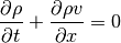
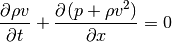
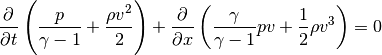
The Euler equations consist of conservation of mass (Eq. (1)), of momentum (Eq. (2)), and of energy (Eq. (3)).
(1)
(2)
(3)
By defining
(4)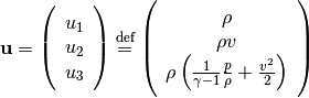
(5)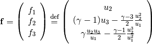
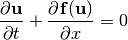
we can rewrite Eqs. (1), (2), and (3) in a general form for nonlinear hyperbolic PDEs:
(6)
The initial condition of the Riemann problem is defined as:
(7)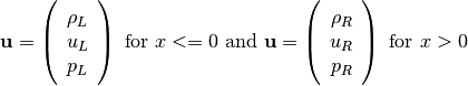
By using Eq. (7), Sod’s initial conditions can be set as:
(8)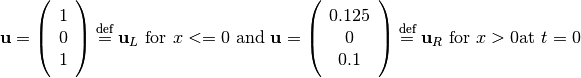
We divide the solution of the problem in “5 zones”. From the left
( ) to the right (
 ) of the diaphragm.
- Region I
- There is no boundary of the tube. The status is always
 .
.
- There is no boundary of the tube. The status is always
- Region II
- Rarefaction wave. The status is continuous from the region 1 to the region 3.
- Region III
- In the shock “pocket”, there is “no more shock” and the hyperbolic PDE
(6) told us
 are Riemann invariants. Together with Rankine-Hugoniot conditions, we know
 and the density is not continuous.
- In the shock “pocket”, there is “no more shock” and the hyperbolic PDE
(6) told us
- Region IV
- Because of the expansion of the shock, there is shock discontinuity. The discontinuity status could be determined by Rankine-Hugoniot conditions [Wesselling01].
- Region V
- There is no boundary of the tube, so the status is always

- There is no boundary of the tube, so the status is always
To derive the analytic solution, we will begin from the region
 to get
 ,
then
,
then  and
finally
and
finally  .
.
Derivation of 
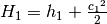
Rankine-Hugoniot conditions gives that the jump conditions must hold across a shock:
(9)
(10)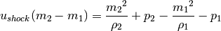
(11)
If this is a stationary shock,  .
(9) tells us
.
(9) tells us  .
.
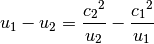
Because and (9),
from (10) we get:
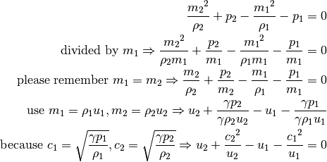
Thus, we get
(12)
Since ,
and (11), we get  .
Use
.
Use  , namely
 and
and 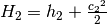 ,
and we could rewrite as
,
and we could rewrite as
Assume  . Because of continuity,
there must be a point with the speed
. Because of continuity,
there must be a point with the speed
 equal to the sound speed
  which satisfies:
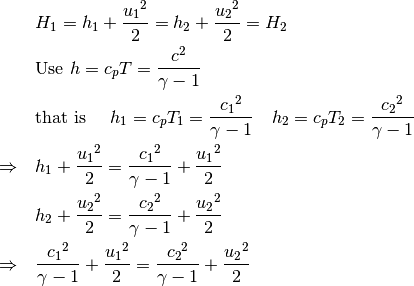
And
(13)
Now let’s try to get
represented by  and
and  .
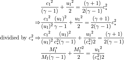
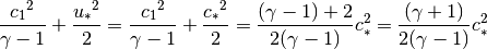
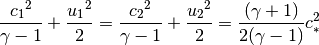
Because of (13)
.
Because of (13)
![& \frac{{c_1}^2}{\gamma - 1} + \frac{{u_1}^2}{2}
= \frac{(\gamma+1)c_{*}}{2(\gamma-1)} \\
& \frac{{c_2}^2}{\gamma - 1} + \frac{{u_2}^2}{2}
= \frac{(\gamma+1)c_{*}}{2(\gamma-1)} \\
\text{multipled by } \frac{(2\gamma-1)}{\gamma{u_1}}
& \text{ and multipled by } \frac{(2\gamma-1)}{\gamma{u_2}}
\text{ seperately} \\
\Rightarrow
& \frac{2{c_1}^2}{\gamma{u_1}} + \frac{{u_1}(\gamma-1)}{\gamma}
= \frac{(\gamma+1)c_{*}}{\gamma{u_1}} \\
& \frac{2{c_2}^2}{\gamma{u_2}} + \frac{{u_2}(\gamma-1)}{\gamma}
= \frac{(\gamma+1)c_{*}}{\gamma{u_2}} \\
\Rightarrow
& \frac{2{c_1}^2}{\gamma{u_1}} =
\frac{(\gamma+1)c_{*}}{\gamma{u_1}} - \frac{{u_1}(\gamma-1)}{\gamma} \\
& \frac{2{c_2}^2}{\gamma{u_2}} =
\frac{(\gamma+1)c_{*}}{\gamma{u_2}} - \frac{{u_2}(\gamma-1)}{\gamma} \\
\Rightarrow
& \frac{{c_1}^2}{\gamma{u_1}}
= \frac{(\gamma+1)c_{*}}{2\gamma{u_1}} - \frac{{u_1}(\gamma-1)}{2\gamma}
= [\frac{(\gamma+1)c_{*}}{\gamma-1}+{u_1}^2]
(\frac{(\gamma-1)}{2\gamma{u_1})}) \\
& \frac{{c_2}^2}{\gamma{u_2}}
= \frac{(\gamma+1)c_{*}}{2\gamma{u_2}} - \frac{{u_2}(\gamma-1)}{2\gamma}
= [\frac{(\gamma+1)c_{*}}{\gamma-1}+{u_2}^2]
(\frac{(\gamma-1)}{2\gamma{u_2})}) \\
\Rightarrow
& \frac{{c_1}^2}{\gamma{u_1}} - \frac{{c_2}^2}{\gamma{u_2}}
= \frac{(\gamma+1)c_{*}}{2\gamma{u_1}} - \frac{{u_1}(\gamma-1)}{2\gamma}
- \frac{(\gamma+1)c_{*}}{2\gamma{u_2}} + \frac{{u_2}(\gamma-1)}{2\gamma}](../_images/math/5ded7ff529a6eb3bf32cb9ab38ba9e08badb69b5.png)
please recall (12), thus
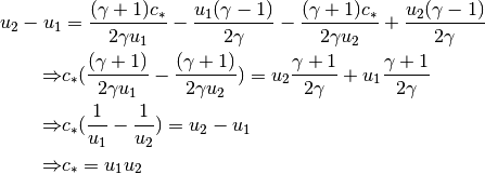
The relation
(14)
is called Prandel-Meyer relation. It means the flow at one side of a shock must be supersonic, and the other side must be subsonic.
Now defining the Mach number  and
and
 , we get from (13):