Formulations (Under Development)
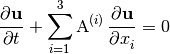
The governing equations of the hydro-acoustic wave include the continuity equation
(1)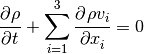
and the momentum equations
(2)![\dpd{\rho v_j}{t}
+ \sum_{i=1}^3 \dpd{(\rho v_iv_j + \delta_{ij}p)}{x_i}
= \dpd{}{x_j}\left(\lambda\sum_{k=1}^3\dpd{v_k}{x_k}\right)
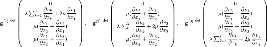
+ \sum_{i=1}^3 \dpd{}{x_i}
\left[\mu \left( \dpd{v_i}{x_j}+\dpd{v_j}{x_i} \right)\right],
\quad j = 1, 2, 3](../_images/math/b2ec40ac04a3db556189321114c47555e0d6dd48.png)
where  is the density,
  and
and  the
Cartesian component of the velocity,
the
Cartesian component of the velocity,  the pressure,
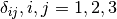 the Kronecker delta,
  the
second viscosity coefficien,
the
second viscosity coefficien,  the dynamic viscosity coefficient,
 the time, and
  , and
, and  the Cartesian
coordinate axes. Newtonian fluid is assumed.
the Cartesian
coordinate axes. Newtonian fluid is assumed.
The above four equations in (1) and (2) have five
independent variables  , and , and hence are
not closed without a constitutive relation. In the
, and , and hence are
not closed without a constitutive relation. In the bulk package,
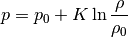
the constitutive relation (or the equation of state) of choice is

where  is a constant and the bulk modulus. We chose to use the
density as the independent variable, and integrate the equation of
state to be
is a constant and the bulk modulus. We chose to use the
density as the independent variable, and integrate the equation of
state to be
(3)
where  and
and  are constants. Substituting (3)
into (2) gives
are constants. Substituting (3)
into (2) gives
(4)![\dpd{\rho v_j}{t} + \sum_{i=1}^3\dpd{}{x_i}
\left[\rho v_iv_j
+ \delta_{ij}\left(p_0 + K\ln\frac{\rho}{\rho_0}\right) \right]
= \sum_{i=1}^3 \dpd{}{x_i}
\left[\delta_{ij} \lambda \sum_{k=1}^3 \dpd{v_k}{x_k}
+ \mu \left( \dpd{v_i}{x_j}+\dpd{v_j}{x_i} \right)\right],
\quad j = 1, 2, 3](../_images/math/833c9dbe62a215b1c9d274def75479be675aaaeb.png)
Jacobian Matrices
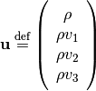
We proceed to analyze the advective part of the governing equations (1) and (4). Define the conservation variables
(5)
and flux functions
(6)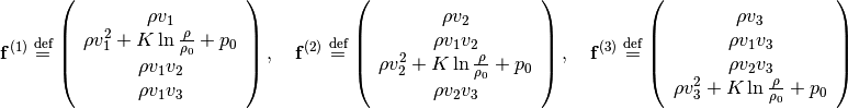
Aided by the definition of conservation variables in (5), the flux
functions defined in (6) can be rewritten with  ,
and
,
and 
(7)
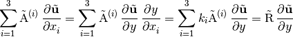
By using (5) and (7), the left-hand-side of the governing equations can be cast into the conservative form
(8)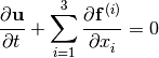
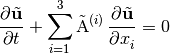
Aided by using the chain rule, (8) can be rewritten in the quasi-linear form
(9)
where the Jacobian matrices  , and
, and
 are defined as
(10)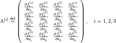
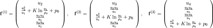
Aided by using (7), the Jacobian matrices defined in (10) can be written out as
(11)
Hyperbolicity
Hyperbolicity is a prerequisite for us to apply the space-time CESE method to a system of first-order PDEs. For the governing equations, (1) and (4), to be hyperbolic, the linear combination of the three Jacobian matrices of their quasi-linear for must be diagonalizable. The spectrum of the linear combination must be all real, too [Warming75], [Chen12].
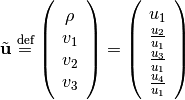
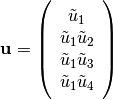
To facilitate the analysis, we chose to use the non-conservative version of the governing equations. Define the non-conservative variables
(12)
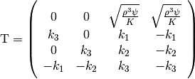
Aided by using (12) and (5), the transformation between the conservative variables and the non-conservative variables can be done with the transformation Jacobian defined as
(13)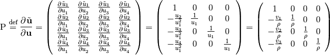
Aided by writing (5) as
the inverse matrix of  can be obtained
(14)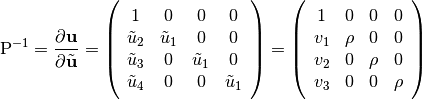
and 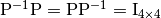 .
.
The transformation matrix can be used to cast the
conservative equations, (9), into non-conservative ones.
Pre-multiplying  to (9) gives
(15)
where
(16)
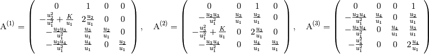
To help obtaining the expression of  , and
, and  , we substitute
(5) into (11) and get
, we substitute
(5) into (11) and get
(17)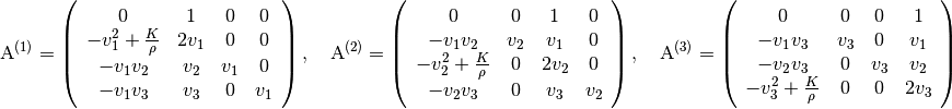
The Jacobian matrices in (16) can be spelled out with the expressions in (13), (14), and (17)
(18)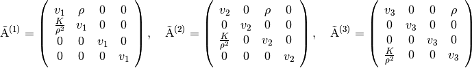
(15) is hyperbolic where the linear combination of its Jacobian
matrices  ,
,  ,
and
,
and
(19)
where  , and
, and  are real and bounded.
The linearly combined Jacobian matrix can be used to rewrite the three-dimensional governing equation, (15), into one-dimensional space
(20)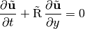
where
(21)
and aided by (19) and the chain rule
The eigenvalues of  can be found by solving the
polynomial equation
can be found by solving the
polynomial equation 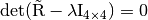 for , and are
(22)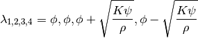
where 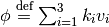 , and
, and  . The corresponding eigenvector matrix is
(23)
The left eigenvector matrix is
(24)
Riemann Invariants
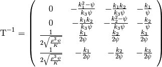
Aided by (23) and (24),
can be diagonalized as
(25)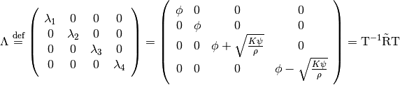
(25) defines the eigenvalue matrix of .
Aach element in the diagonal of the eigenvalue matrix is the eigenvalue listed
in (22). Pre-multiplying (20) with
 gives
gives
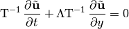
Define the characteristic variables
(26)
such that

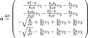
Then aided by the chain rule, we can write
(27)
The components of  defined in (26) are the
Riemann invariants.
defined in (26) are the
Riemann invariants.
![\sum_{i=1}^3 \dpd{}{x_i}
\left[\delta_{ij} \lambda \sum_{k=1}^3 \dpd{v_k}{x_k}
+ \mu \left( \dpd{v_i}{x_j}+\dpd{v_j}{x_i} \right)\right],
\quad j = 1, 2, 3](../_images/math/c180106122bc5d5f64dce16735cf1db512a90bd2.png)