Viscoelastic Wave (Under Development)
Mathematical Model
For isothermal viscoelastic material, the model equations consist conservation of mass and momentum as follows,
(1)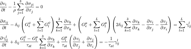
where  are the Cartesian component of the velocity,
  the
density,
the
density,  the stress tensor,
  the
internal variables, and
the
internal variables, and  the Kronecker delta. Subscripts
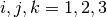 are for the Cartesian tensors.
  , and
, and  are the constants of the
standard linear solid (SLS) model with
are the constants of the
standard linear solid (SLS) model with 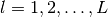 .
.  is the number of the employed SLS model components.
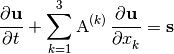
Equation (1) can be further organized to a vector form:
(2)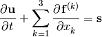
where  is the solution variable,
  ,
,
 , and
, and  flux functions, and
 the source term.
Jacobian Matrices
By applying the chain rule to Eq. (2), we can derive the Jacobian matrices:
(3)
where  ,
,  , and
, and
 are
are 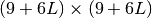 are the Jacobian
matrices:
are the Jacobian
matrices:
(4)
where
![\mathrm{B}^{(i)} \defeq \left( \begin{array}{ccc}
\left[ 2(G^{\mu}_e + \sum^L_{l=1} G^{\mu}_l)
- (G^{\psi}_e + \sum^L_{l=1} G^{\psi}_l) \right]
\mathrm{M}^{(i)}
- (G^{\psi}_e+\sum^L_{l=1}G^{\psi}_l) \mathrm{K}^{(i)}
\\
\frac{G^{\phi}_1 - G^{\mu}_1}{\tau_{\sigma 1}} \mathrm{M}^{(i)}
+ \frac{G^{\phi}_1}{\tau_{\sigma 1}} \mathrm{N}^{(i)}
+ \frac{G^{\mu}_1}{\tau_{\sigma 1}} \mathrm{K}^{(i)}
\\
\vdots \\
\frac{G^{\phi}_L - G^{\mu}_L}{\tau_{\sigma 1}} \mathrm{M}^{(i)}
+ \frac{G^{\phi}_L}{\tau_{\sigma 1}} \mathrm{N}^{(i)}
+ \frac{G^{\mu}_L}{\tau_{\sigma 1}} \mathrm{K}^{(i)}
\end{array} \right), \,
\mathrm{C}^{(i)} \defeq -\frac{1}{\rho} {\mathrm{K}^{(i)}}^t,
\quad i = 1, 2, 3](_images/math/c95d3dede162b508b37db046fd92f7265bb93ed3.png)
and
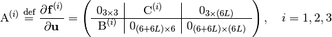
(5)
(6)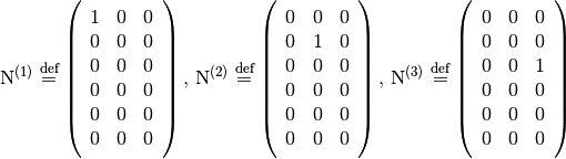
(7)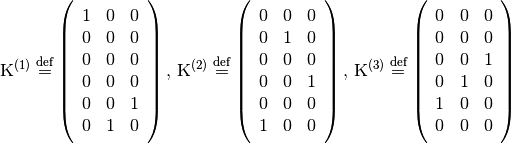
 ,
,  , and
, and
 are
are  matrices.
 ,
,  , and
, and
 are
are  matrices.
Hyperbolicity
The left hand side of the model equation Eq. (3) can be proved as a hyperbolic system. The method of proof is similar to the Hydro-Acoustics (Under Development). The list of the eigenvalues is provided:
(8)
where  , and
, and
 . The
. The  , and
, and
 are the components of a direction vector, as used in
Hydro-Acoustics (Under Development).
are the components of a direction vector, as used in
Hydro-Acoustics (Under Development).